bruceR - 统计分析工具

R包

统计分析

数据处理

Published

January 10, 2025

R包介绍

bruceR 全称 “BRoadly Useful Convenient and Efficient R functions”，由包寒吴霜博士开发，是一个集成了众多实用功能的 R 包，专为科研数据分析设计。

链接：CRAN | GitHub | 中文教程

核心功能

bruceR 涵盖了数据分析的完整流程：

模块	功能	主要函数
基础编程	路径设置、数据导入导出、表格打印	`set.wd()`, `import()`, `export()`, `print_table()`
数据计算	量表计算、反向计分、重编码	`MEAN()`, `SUM()`, `RECODE()`, `RESCALE()`
信效度分析	信度分析、因子分析	`Alpha()`, `EFA()`, `PCA()`, `CFA()`
描述统计	描述统计、频率分析、相关分析	`Describe()`, `Freq()`, `Corr()`
方差分析	t检验、ANOVA、简单效应、事后比较	`TTEST()`, `MANOVA()`, `EMMEANS()`
回归模型	模型汇总、多层模型	`model_summary()`, `HLM_summary()`
中介调节	PROCESS 宏	`PROCESS()`, `med_summary()`

依赖包自动加载

加载 bruceR 时会自动加载常用包：

数据处理：data.table, dplyr, tidyr, stringr
可视化：ggplot2
统计分析：psych, emmeans, lmerTest, effectsize, performance

R包安装

# 方法1：从 CRAN 安装（推荐）
install.packages("bruceR", dep = TRUE)

# 方法2：从 GitHub 安装最新版
install.packages("devtools")
devtools::install_github("psychbruce/bruceR", dep = TRUE, force = TRUE)

library(bruceR)

基础编程功能

set.wd()：智能设置工作目录

自动将工作目录设置为当前脚本所在路径：

set.wd()

import() / export()：万能数据导入导出

支持几乎所有常见数据格式，自动识别文件类型：

# 支持的格式：
# - 文本：.txt, .csv, .tsv
# - Excel：.xls, .xlsx
# - SPSS：.sav
# - Stata：.dta
# - R对象：.rda, .rds, .RData

# 导入数据
data <- import("data.xlsx")
data <- import("data.sav")
data <- import("data.dta")

# 导出数据
export(data, file = "output.xlsx")
export(data, file = "output.csv")

cc()：快速创建字符向量

比 c() 更简洁，无需引号：

# 传统写法
c("age", "gender", "education")

[1] "age"       "gender"    "education"

# bruceR 写法
cc("age, gender, education")

[1] "age"       "gender"    "education"

print_table()：生成三线表

summary_data <- data.frame(
  Variable = c("Age", "Income", "Score"),
  Mean = c(35.2, 5000, 78.5),
  SD = c(8.3, 1200, 12.1),
  N = c(100, 100, 100)
)

print_table(summary_data)

─────────────────────────────────────
   Variable     Mean       SD       N
─────────────────────────────────────
1    Age      35.200    8.300 100.000
2    Income 5000.000 1200.000 100.000
3    Score    78.500   12.100 100.000
─────────────────────────────────────

数据计算功能

MEAN() / SUM()：横向计算（支持反向计分）

心理学量表经常需要计算多个题目的均值或总分，并处理反向计分：

# 创建模拟问卷数据（5点量表，共6题）
set.seed(42)
questionnaire <- data.frame(
  id = 1:5,
  q1 = sample(1:5, 5, replace = TRUE),
  q2 = sample(1:5, 5, replace = TRUE),
  q3 = sample(1:5, 5, replace = TRUE),
  q4 = sample(1:5, 5, replace = TRUE),
  q5 = sample(1:5, 5, replace = TRUE),
  q6 = sample(1:5, 5, replace = TRUE)
)
questionnaire

  id q1 q2 q3 q4 q5 q6
1  1  1  4  1  3  5  4
2  2  5  2  5  1  5  3
3  3  1  2  4  1  5  2
4  4  1  1  2  3  4  1
5  5  2  4  2  4  2  2

# 计算均值（q3、q6 反向计分，量表范围1-5）
questionnaire$score_mean <- MEAN(
  questionnaire, 
  varrange = "q1:q6",
  rev = c("q3", "q6"),
  likert = 1:5
)

# 计算总分
questionnaire$score_sum <- SUM(
  questionnaire, 
  varrange = "q1:q6",
  rev = c("q3", "q6"),
  likert = 1:5
)

questionnaire[, c("id", "score_mean", "score_sum")]

  id score_mean score_sum
1  1   3.333333        20
2  2   2.833333        17
3  3   2.500000        15
4  4   3.000000        18
5  5   3.333333        20

RECODE()：变量重编码

d <- data.frame(age = c(18, 25, 35, 45, 55, 65, 75))

d$age_group <- RECODE(d$age, 
  "lo:29 = '青年'; 
   30:59 = '中年'; 
   60:hi = '老年'"
)
d

  age age_group
1  18      青年
2  25      青年
3  35      中年
4  45      中年
5  55      中年
6  65      老年
7  75      老年

RESCALE()：变量标准化

scores <- c(2, 3, 4, 5, 6, 7, 8)
RESCALE(scores, to = 0:100)

[1]   0.00000  16.66667  33.33333  50.00000  66.66667  83.33333 100.00000

信度与因子分析

Alpha()：信度分析

data("bfi", package = "psych")

# Alpha 需要指定数据和变量名
Alpha(bfi, var = "A", items = 1:5)


Reliability Analysis

Summary:
Total Items: 5
Scale Range: 1 ~ 6
Total Cases: 2800
Valid Cases: 2709 (96.8%)

Scale Statistics:
Mean = 4.208
S.D. = 0.735
Cronbach’s α = 0.431
McDonald’s ω = 0.592

Warning: Scale reliability is low. You may check item codings.
Item A1 correlates negatively with the scale and may be reversed.
You can specify this argument: rev=c("A1")

Item Statistics (Cronbach’s α If Item Deleted):
─────────────────────────────────────────────
     Mean    S.D. Item-Rest Cor. Cronbach’s α
─────────────────────────────────────────────
A1  2.412 (1.405)         -0.311        0.718
A2  4.797 (1.176)          0.372        0.278
A3  4.599 (1.305)          0.478        0.174
A4  4.682 (1.486)          0.365        0.252
A5  4.551 (1.262)          0.448        0.207
─────────────────────────────────────────────
Item-Rest Cor. = Corrected Item-Total Correlation

EFA()：探索性因子分析

data("bfi", package = "psych")

# 探索性因子分析：使用 var + items 格式
# 分析外向性(E)量表的5个题目
EFA(bfi, var = "E", items = 1:5, nfactors = 2, plot.scree = FALSE)


Principal Component Analysis

Summary:
Total Items: 5
Scale Range: 1 ~ 6
Total Cases: 2800
Valid Cases: 2713 (96.9%)

Extraction Method:
- Principal Component Analysis
Rotation Method:
- Varimax (with Kaiser Normalization)

KMO and Bartlett's Test:
- Kaiser-Meyer-Olkin (KMO) Measure of Sampling Adequacy: MSA = 0.799
- Bartlett's Test of Sphericity: Approx. χ²(10) = 3011.40, p < 1e-99 ***

Total Variance Explained:
──────────────────────────────────────────────────────────────────────────────────
             Eigenvalue Variance % Cumulative % SS Loading Variance % Cumulative %
──────────────────────────────────────────────────────────────────────────────────
Component 1       2.565     51.298       51.298      1.884     37.680       37.680
Component 2       0.768     15.368       66.666      1.449     28.986       66.666
Component 3       0.643     12.851       79.517                                   
Component 4       0.561     11.211       90.728                                   
Component 5       0.464      9.272      100.000                                   
──────────────────────────────────────────────────────────────────────────────────

Component Loadings (Rotated) (Sorted by Size):
─────────────────────────────
       RC1    RC2 Communality
─────────────────────────────
E1   0.812 -0.098       0.668
E2   0.752 -0.304       0.658
E4  -0.736  0.290       0.625
E5  -0.145  0.860       0.761
E3  -0.312  0.723       0.620
─────────────────────────────
Communality = Sum of Squared (SS) Factor Loadings
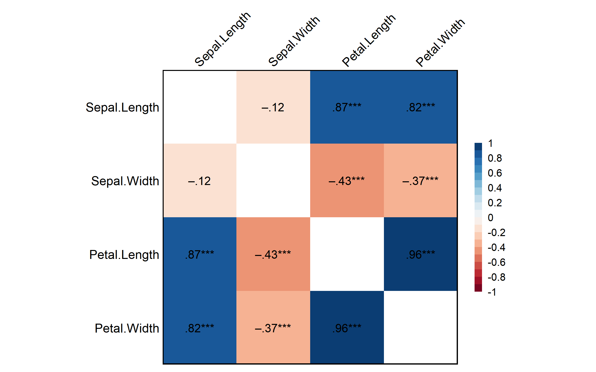
(Uniqueness = 1 - Communality)

描述统计与相关分析

Describe()：描述统计

Describe(iris[, 1:4])

Descriptive Statistics:
────────────────────────────────────────────────────────────────
                N Mean   SD | Median  Min  Max Skewness Kurtosis
────────────────────────────────────────────────────────────────
Sepal.Length  150 5.84 0.83 |   5.80 4.30 7.90     0.31    -0.61
Sepal.Width   150 3.06 0.44 |   3.00 2.00 4.40     0.31     0.14
Petal.Length  150 3.76 1.77 |   4.35 1.00 6.90    -0.27    -1.42
Petal.Width   150 1.20 0.76 |   1.30 0.10 2.50    -0.10    -1.36
────────────────────────────────────────────────────────────────

Freq()：频率分析

Freq(iris$Species)

Frequency Statistics:
───────────────────
             N    %
───────────────────
setosa      50 33.3
versicolor  50 33.3
virginica   50 33.3
───────────────────
Total N = 150

Corr()：相关分析

Corr(iris[, 1:4])

Pearson's r and 95% confidence intervals:
─────────────────────────────────────────────────────────────
                               r       [95% CI]     p       N
─────────────────────────────────────────────────────────────
Sepal.Length-Sepal.Width   -0.12 [-0.27,  0.04]  .152     150
Sepal.Length-Petal.Length   0.87 [ 0.83,  0.91] <.001 *** 150
Sepal.Length-Petal.Width    0.82 [ 0.76,  0.86] <.001 *** 150
Sepal.Width-Petal.Length   -0.43 [-0.55, -0.29] <.001 *** 150
Sepal.Width-Petal.Width    -0.37 [-0.50, -0.22] <.001 *** 150
Petal.Length-Petal.Width    0.96 [ 0.95,  0.97] <.001 *** 150
─────────────────────────────────────────────────────────────

统计检验

TTEST()：t检验

# 独立样本 t 检验（需要两水平因子）
iris_subset <- iris[iris$Species %in% c("versicolor", "virginica"), ]
iris_subset$Species <- droplevels(iris_subset$Species)

TTEST(iris_subset, y = "Sepal.Length", x = "Species")


Independent-Samples t-test

Hypothesis: two-sided (μ2 - μ1 ≠ 0)

Descriptives:
───────────────────────────────────────────────
     Variable  Factor      Level  N Mean (S.D.)
───────────────────────────────────────────────
 Sepal.Length Species versicolor 50 5.94 (0.52)
 Sepal.Length Species virginica  50 6.59 (0.64)
───────────────────────────────────────────────

Levene’s test for homogeneity of variance:
────────────────────────────────────────────────────────────────────────────
                                                Levene’s F df1 df2     p    
────────────────────────────────────────────────────────────────────────────
Sepal.Length: Species (virginica - versicolor)        1.42   1  98  .236    
────────────────────────────────────────────────────────────────────────────
Note: H0 = equal variance (homoscedasticity).
If significant (violation of the assumption),
then you should better set `var.equal=FALSE`.

Results of t-test:
─────────────────────────────────────────────────────────────────────────────────────────────────────────────────
                                                   t df     p     Difference [95% CI] Cohen’s d [95% CI]     BF10
─────────────────────────────────────────────────────────────────────────────────────────────────────────────────
Sepal.Length: Species (virginica - versicolor)  5.63 98 <.001 ***   0.65 [0.42, 0.88]  1.13 [0.73, 1.52] 7.04e+04
─────────────────────────────────────────────────────────────────────────────────────────────────────────────────

MANOVA()：多因素方差分析

MANOVA(data = npk, dv = "yield", between = c("N", "P", "K"))


====== ANOVA (Between-Subjects Design) ======

Descriptives:
─────────────────────────────
 "N" "P" "K"   Mean    S.D. n
─────────────────────────────
  N0  P0  K0 51.433 (4.600) 3
  N0  P0  K1 52.000 (5.635) 3
  N0  P1  K0 54.333 (9.411) 3
  N0  P1  K1 50.500 (2.364) 3
  N1  P0  K0 63.767 (5.086) 3
  N1  P0  K1 54.667 (4.216) 3
  N1  P1  K0 57.933 (5.478) 3
  N1  P1  K1 54.367 (5.006) 3
─────────────────────────────
Total sample size: N = 24

ANOVA Table:
Dependent variable(s):      yield
Between-subjects factor(s): N, P, K
Within-subjects factor(s):  –
Covariate(s):               –
──────────────────────────────────────────────────────────────────────────
                MS    MSE df1 df2     F     p     η²p [90% CI of η²p]  η²G
──────────────────────────────────────────────────────────────────────────
N          189.282 30.724   1  16 6.161  .025 *     .278 [.024, .529] .278
P            8.402 30.724   1  16 0.273  .608       .017 [.000, .220] .017
K           95.202 30.724   1  16 3.099  .097 .     .162 [.000, .427] .162
N * P       21.282 30.724   1  16 0.693  .418       .041 [.000, .277] .041
N * K       33.135 30.724   1  16 1.078  .314       .063 [.000, .312] .063
P * K        0.482 30.724   1  16 0.016  .902       .001 [.000, .078] .001
N * P * K   37.002 30.724   1  16 1.204  .289       .070 [.000, .322] .070
──────────────────────────────────────────────────────────────────────────
MSE = mean square error (the residual variance of the linear model)
η²p = partial eta-squared = SS / (SS + SSE) = F * df1 / (F * df1 + df2)
ω²p = partial omega-squared = (F - 1) * df1 / (F * df1 + df2 + 1)
η²G = generalized eta-squared (see Olejnik & Algina, 2003)
Cohen’s f² = η²p / (1 - η²p)

Levene’s Test for Homogeneity of Variance:
───────────────────────────────────────
           Levene’s F df1 df2     p    
───────────────────────────────────────
DV: yield       0.986   7  16  .475    
───────────────────────────────────────

EMMEANS()：边际均值与事后比较

result <- MANOVA(npk, dv = "yield", between = c("N", "P"))


====== ANOVA (Between-Subjects Design) ======

Descriptives:
─────────────────────────
 "N" "P"   Mean    S.D. n
─────────────────────────
  N0  P0 51.717 (4.611) 6
  N0  P1 52.417 (6.486) 6
  N1  P0 59.217 (6.504) 6
  N1  P1 56.150 (5.084) 6
─────────────────────────
Total sample size: N = 24

ANOVA Table:
Dependent variable(s):      yield
Between-subjects factor(s): N, P
Within-subjects factor(s):  –
Covariate(s):               –
──────────────────────────────────────────────────────────────────────
            MS    MSE df1 df2     F     p     η²p [90% CI of η²p]  η²G
──────────────────────────────────────────────────────────────────────
N      189.282 32.870   1  20 5.758  .026 *     .224 [.017, .460] .224
P        8.402 32.870   1  20 0.256  .619       .013 [.000, .181] .013
N * P   21.282 32.870   1  20 0.647  .430       .031 [.000, .230] .031
──────────────────────────────────────────────────────────────────────
MSE = mean square error (the residual variance of the linear model)
η²p = partial eta-squared = SS / (SS + SSE) = F * df1 / (F * df1 + df2)
ω²p = partial omega-squared = (F - 1) * df1 / (F * df1 + df2 + 1)
η²G = generalized eta-squared (see Olejnik & Algina, 2003)
Cohen’s f² = η²p / (1 - η²p)

Levene’s Test for Homogeneity of Variance:
───────────────────────────────────────
           Levene’s F df1 df2     p    
───────────────────────────────────────
DV: yield       0.160   3  20  .922    
───────────────────────────────────────

EMMEANS(result, effect = "N")

------ EMMEANS (effect = "N") ------

Joint Tests of "N":
───────────────────────────────────────────────────
 Effect df1 df2     F     p     η²p [90% CI of η²p]
───────────────────────────────────────────────────
  N       1  20 5.758  .026 *     .224 [.017, .460]
  P       1  20 0.256  .619       .013 [.000, .181]
  N * P   1  20 0.647  .430       .031 [.000, .230]
───────────────────────────────────────────────────
Note. Simple effects of repeated measures with 3 or more levels
are different from the results obtained with SPSS MANOVA syntax.

Univariate Tests of "N":
────────────────────────────────────────────────────────
           Sum of Squares df Mean Square     F     p    
────────────────────────────────────────────────────────
Mean: "N"         189.282  1     189.282 5.758  .026 *  
Residuals         657.400 20      32.870                
────────────────────────────────────────────────────────
Note. Identical to the results obtained with SPSS GLM EMMEANS syntax.

Estimated Marginal Means of "N":
────────────────────────────────────
 "N"   Mean [95% CI of Mean]    S.E.
────────────────────────────────────
  N0 52.067 [48.614, 55.519] (1.655)
  N1 57.683 [54.231, 61.136] (1.655)
────────────────────────────────────

Pairwise Comparisons of "N":
─────────────────────────────────────────────────────────────────────
 Contrast Estimate    S.E. df     t     p     Cohen’s d [95% CI of d]
─────────────────────────────────────────────────────────────────────
  N1 - N0    5.617 (2.341) 20 2.400  .026 *      0.980 [0.128, 1.831]
─────────────────────────────────────────────────────────────────────
Pooled SD for computing Cohen’s d: 5.733
Results are averaged over the levels of: P
No need to adjust p values.

Disclaimer:
By default, pooled SD is Root Mean Square Error (RMSE).
There is much disagreement on how to compute Cohen’s d.
You are completely responsible for setting `sd.pooled`.
You might also use `effectsize::t_to_d()` to compute d.

回归分析

model_summary()：模型汇总

lm1 <- lm(Sepal.Length ~ Sepal.Width, data = iris)
lm2 <- lm(Sepal.Length ~ Sepal.Width + Petal.Length, data = iris)
lm3 <- lm(Sepal.Length ~ Sepal.Width + Petal.Length + Petal.Width, data = iris)

# 多个模型对比
model_summary(list(lm1, lm2, lm3))


Model Summary

──────────────────────────────────────────────────────────────────
              (1) Sepal.Length  (2) Sepal.Length  (3) Sepal.Length
──────────────────────────────────────────────────────────────────
(Intercept)     6.526 ***         2.249 ***         1.856 ***     
               (0.479)           (0.248)           (0.251)        
Sepal.Width    -0.223             0.596 ***         0.651 ***     
               (0.155)           (0.069)           (0.067)        
Petal.Length                      0.472 ***         0.709 ***     
                                 (0.017)           (0.057)        
Petal.Width                                        -0.556 ***     
                                                   (0.128)        
──────────────────────────────────────────────────────────────────
R^2             0.014             0.840             0.859         
Adj. R^2        0.007             0.838             0.856         
Num. obs.     150               150               150             
──────────────────────────────────────────────────────────────────
Note. * p < .05, ** p < .01, *** p < .001.

# 输出标准化系数
model_summary(lm3, std = TRUE)


Model Summary

──────────────────────────────
              (1) Sepal.Length
──────────────────────────────
Sepal.Width      .343 ***     
                (.035)        
Petal.Length    1.512 ***     
                (.121)        
Petal.Width     -.512 ***     
                (.117)        
──────────────────────────────
R^2              .859         
Adj. R^2         .856         
Num. obs.     150             
──────────────────────────────
Note. * p < .05, ** p < .01, *** p < .001.

# Check for Multicollinearity

Low Correlation

        Term  VIF     VIF 95% CI adj. VIF Tolerance Tolerance 95% CI
 Sepal.Width 1.27 [ 1.11,  1.65]     1.13      0.79     [0.61, 0.90]

High Correlation

         Term   VIF     VIF 95% CI adj. VIF Tolerance Tolerance 95% CI
 Petal.Length 15.10 [11.27, 20.36]     3.89      0.07     [0.05, 0.09]
  Petal.Width 14.23 [10.63, 19.19]     3.77      0.07     [0.05, 0.09]

中介与调节分析

PROCESS()：中介调节分析

set.seed(123)
n <- 200
mediation_data <- data.frame(
  X = rnorm(n),
  M = rnorm(n),
  Y = rnorm(n)
)
mediation_data$M <- 0.5 * mediation_data$X + rnorm(n, sd = 0.5)
mediation_data$Y <- 0.4 * mediation_data$M + 0.3 * mediation_data$X + rnorm(n, sd = 0.5)

# 简单中介模型
PROCESS(mediation_data, y = "Y", x = "X", meds = "M", 
        ci = "boot", nsim = 100)


****************** PART 1. Regression Model Summary ******************

PROCESS Model ID : 4
Model Type : Simple Mediation
-    Outcome (Y) : Y
-  Predictor (X) : X
-  Mediators (M) : M
- Moderators (W) : -
- Covariates (C) : -
-   HLM Clusters : -

All numeric predictors have been grand-mean centered.
(For details, please see the help page of PROCESS.)

Formula of Mediator:
-    M ~ X
Formula of Outcome:
-    Y ~ X + M

CAUTION:
  Fixed effect (coef.) of a predictor involved in an interaction
  denotes its "simple effect/slope" at the other predictor = 0.
  Only when all predictors in an interaction are mean-centered
  can the fixed effect be interpreted as "main effect"!
  
Model Summary

──────────────────────────────────────────────────
             (1) Y        (2) M        (3) Y      
──────────────────────────────────────────────────
(Intercept)    0.010       -0.015        0.010    
              (0.039)      (0.036)      (0.037)   
X              0.462 ***    0.475 ***    0.302 ***
              (0.041)      (0.039)      (0.052)   
M                                        0.336 ***
                                        (0.072)   
──────────────────────────────────────────────────
R^2            0.391        0.434        0.452    
Adj. R^2       0.388        0.431        0.446    
Num. obs.    200          200          200        
──────────────────────────────────────────────────
Note. * p < .05, ** p < .01, *** p < .001.

************ PART 2. Mediation/Moderation Effect Estimate ************

Package Use : ‘mediation’ (v4.5.1)
Effect Type : Simple Mediation (Model 4)
Sample Size : 200
Random Seed : set.seed()
Simulations : 100 (Bootstrap)


Running 100 simulations...
Indirect Path: "X" (X) ==> "M" (M) ==> "Y" (Y)
─────────────────────────────────────────────────────────────
               Effect    S.E.      z     p      [Boot 95% CI]
─────────────────────────────────────────────────────────────
Indirect (ab)   0.160 (0.034)  4.692 <.001 *** [0.107, 0.235]
Direct (c')     0.302 (0.051)  5.932 <.001 *** [0.194, 0.386]
Total (c)       0.462 (0.041) 11.288 <.001 *** [0.368, 0.529]
─────────────────────────────────────────────────────────────
Percentile Bootstrap Confidence Interval
(SE and CI are estimated based on 100 Bootstrap samples.)

Note. The results based on bootstrapping or other random processes
are unlikely identical to other statistical software (e.g., SPSS).
To make results reproducible, you need to set a seed (any number).
Please see the help page for details: help(PROCESS)
Ignore this note if you have already set a seed. :)

其他实用功能

运算符

# %notin%：不在其中
c(1, 2, 3) %notin% c(2, 4, 6)

[1]  TRUE FALSE  TRUE

# %allin%：全部在其中
c(1, 2) %allin% c(1, 2, 3, 4)

[1] TRUE

theme_bruce()：ggplot2 主题

library(ggplot2)

ggplot(iris, aes(x = Sepal.Length, y = Sepal.Width, color = Species)) +
  geom_point(size = 2, alpha = 0.7) +
  geom_smooth(method = "lm", se = FALSE) +
  labs(title = "鸢尾花数据可视化") +
  theme_bruce()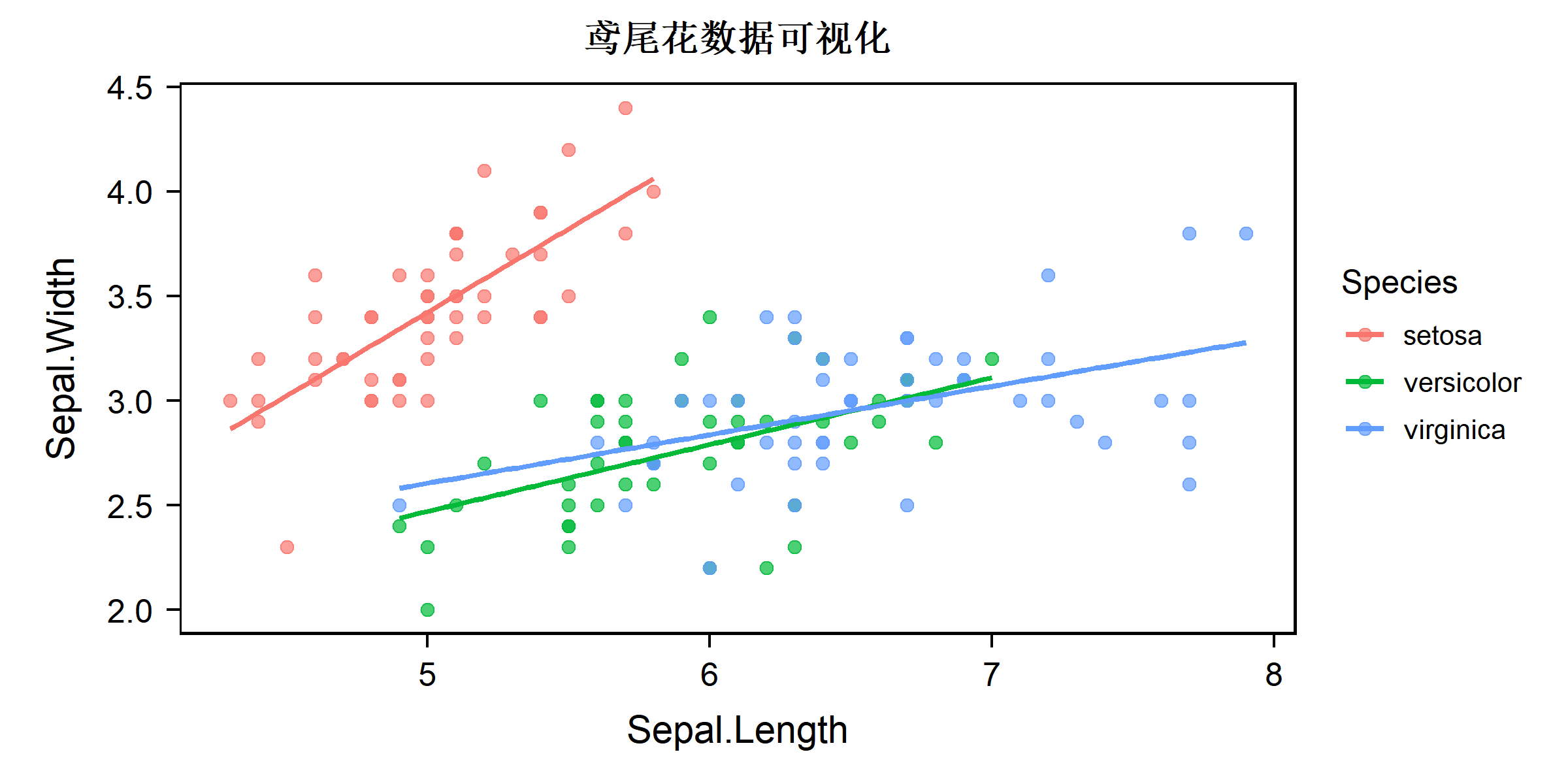

导出到 Word

bruceR 的一大特色是可以将结果直接导出到 Word 文档：

# 描述统计
Describe(iris[, 1:4], file = "descriptives.doc")

# 相关矩阵
Corr(iris[, 1:4], file = "correlation.doc")

# 回归模型
model_summary(list(lm1, lm2, lm3), file = "regression.doc")

# 中介分析
PROCESS(data, y = "Y", x = "X", meds = "M", file = "mediation.doc")

函数速查表

类别	函数	功能
基础	`set.wd()`	设置工作目录到当前脚本位置
	`import()` / `export()`	万能数据导入/导出
	`cc()`	快速创建字符向量
	`print_table()`	打印三线表
计算	`MEAN()` / `SUM()`	横向计算（支持反向计分）
	`RECODE()`	变量重编码
	`RESCALE()`	变量标准化
信效度	`Alpha()`	Cronbach’s α 信度分析
	`EFA()` / `PCA()`	探索性因子分析/主成分分析
	`CFA()`	验证性因子分析
描述	`Describe()`	描述统计
	`Freq()`	频率分析与交叉表
	`Corr()`	相关分析与热力图
检验	`TTEST()`	t检验（单样本/独立/配对）
	`MANOVA()`	多因素方差分析
	`EMMEANS()`	边际均值与事后比较
回归	`model_summary()`	回归模型整洁输出
	`GLM_summary()`	广义线性模型汇总
	`HLM_summary()`	多层线性模型汇总
中介	`PROCESS()`	中介/调节效应分析
	`med_summary()`	中介效应汇总

参考资源

bruceR GitHub 主页
CRAN 官方页面
中文教程：概述篇
中文教程：常见问题
引用：Bao, H. W. S. (2021). bruceR: Broadly useful convenient and efficient R functions. https://doi.org/10.32614/CRAN.package.bruceR