library(ggplot2)
library(cowplot)
library(dplyr)cowplot: 专业图形组合与美化
可视化
ggplot2扩展
简介
cowplot 是 ggplot2 的扩展包,专注于:
- 专业主题:出版级简洁主题
- 图形组合:灵活的多图排列
- 图形嵌入:在图中添加子图
- 标签注释:自动添加 A/B/C 面板标签
- 对齐控制:精确对齐多图坐标轴
主题系统
theme_cowplot - 经典主题
p <- ggplot(mtcars, aes(wt, mpg)) +
  geom_point(aes(color = factor(cyl)), size = 3)

# cowplot 经典主题:无网格线,粗坐标轴
p + theme_cowplot(font_size = 12)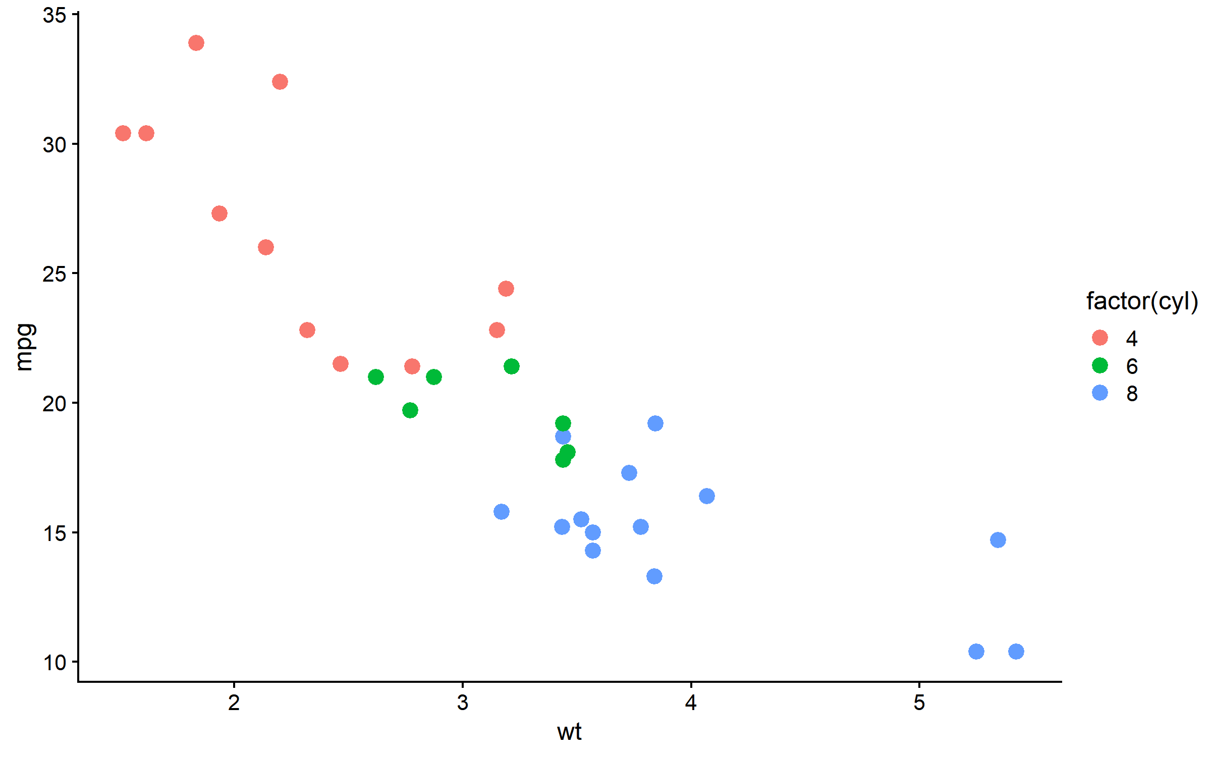
theme_minimal_grid - 极简网格
p + theme_minimal_grid(font_size = 12)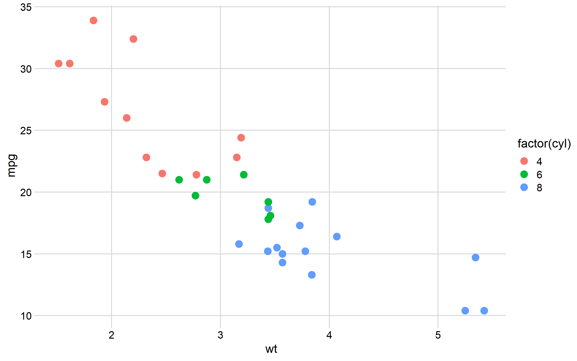
theme_minimal_hgrid / vgrid
p1 <- p + theme_minimal_hgrid() + ggtitle("水平网格")
p2 <- p + theme_minimal_vgrid() + ggtitle("垂直网格")
plot_grid(p1, p2, ncol = 2)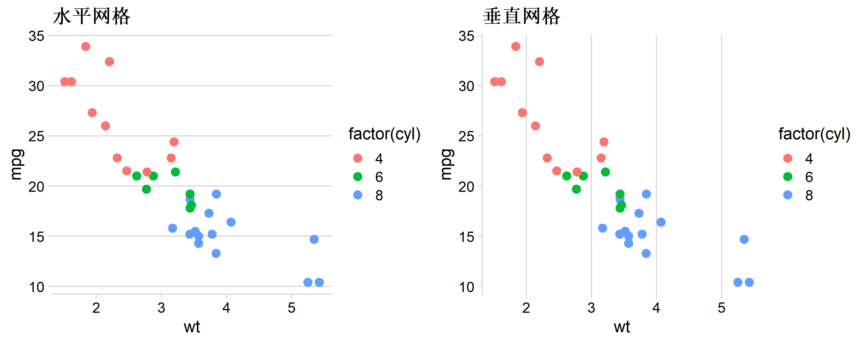
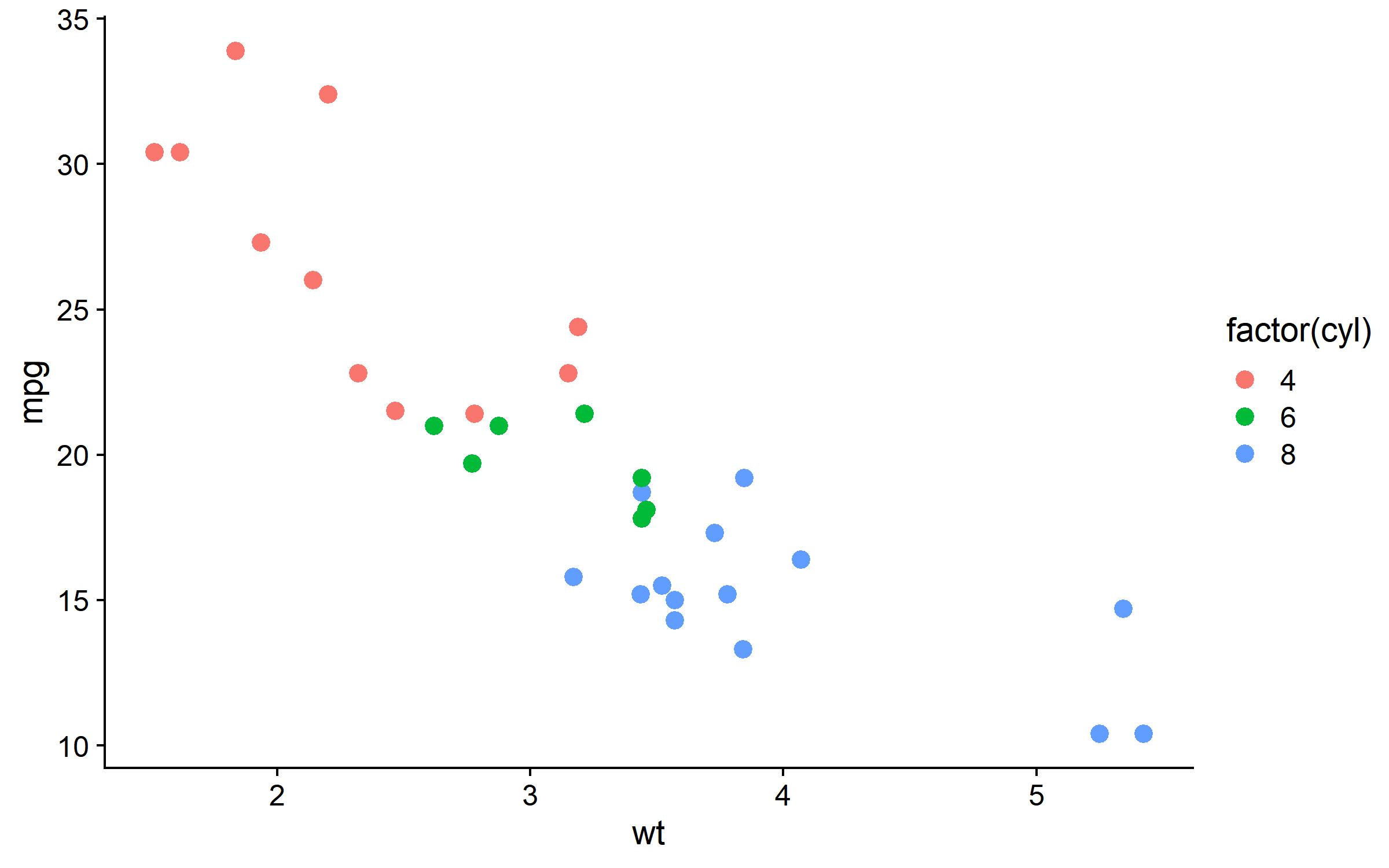
theme_half_open - 半开放坐标轴
# 只显示左下坐标轴,适合科研图
p + theme_half_open(font_size = 12)
主题参数详解
p + theme_cowplot(
  font_size = 14,       # 基础字号
  font_family = "",     # 字体
  line_size = 0.5,      # 线条粗细
  rel_small = 12/14,    # 小字号比例
  rel_tiny = 10/14,     # 更小字号比例
  rel_large = 16/14     # 大字号比例
)
图形组合:plot_grid()
基础组合
p1 <- ggplot(mtcars, aes(wt, mpg)) + geom_point() + theme_cowplot()
p2 <- ggplot(mtcars, aes(disp, mpg)) + geom_point() + theme_cowplot()
p3 <- ggplot(mtcars, aes(factor(cyl))) + geom_bar(fill = "steelblue") + theme_cowplot()
p4 <- ggplot(mtcars, aes(hp, mpg)) + geom_point() + theme_cowplot()

# 2x2 网格
plot_grid(p1, p2, p3, p4, ncol = 2)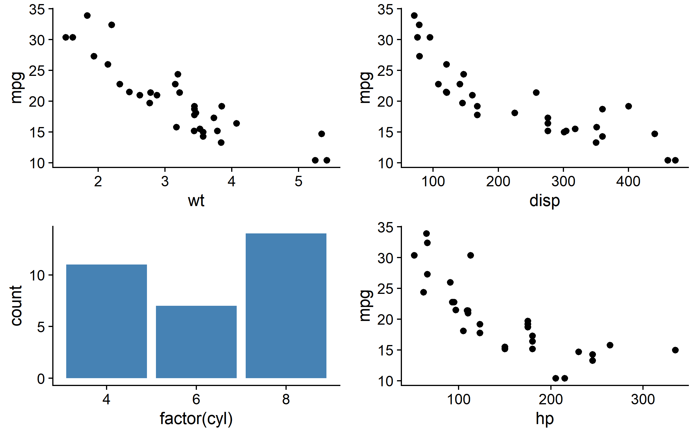
添加标签
# A/B/C/D 标签
plot_grid(
  p1, p2, p3, p4,
  ncol = 2,
  labels = "AUTO",          # 自动 A/B/C/D
  label_size = 14,          # 标签字号
  label_fontface = "bold"   # 粗体
)
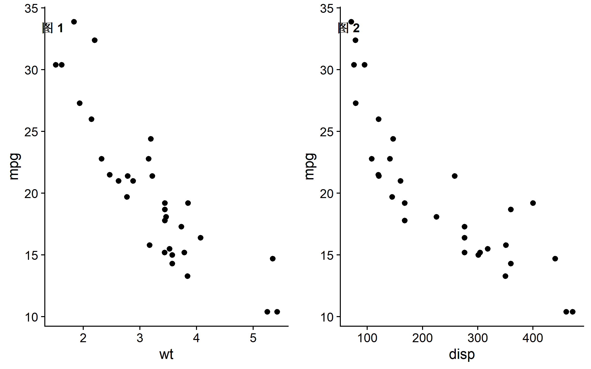
# 自定义标签
plot_grid(
  p1, p2,
  labels = c("图 1", "图 2"),
  label_size = 12,
  label_x = 0.1,   # 标签 x 位置 (0-1)
  label_y = 0.95   # 标签 y 位置 (0-1)
)
控制相对大小
# rel_widths 控制列宽比例
plot_grid(p1, p3, ncol = 2, rel_widths = c(2, 1))  # 左:右 = 2:1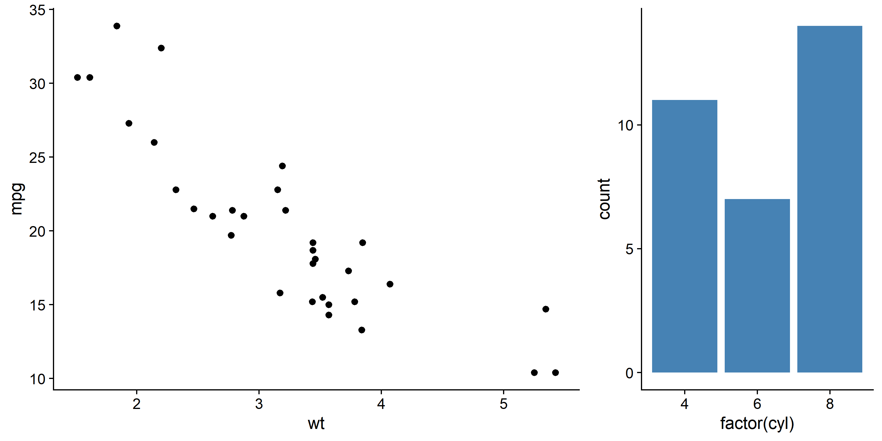
# rel_heights 控制行高比例
plot_grid(p1, p3, nrow = 2, rel_heights = c(2, 1))  # 上:下 = 2:1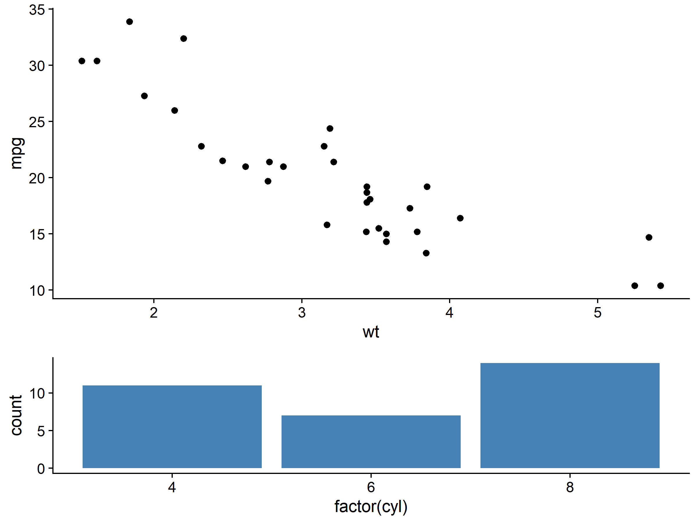
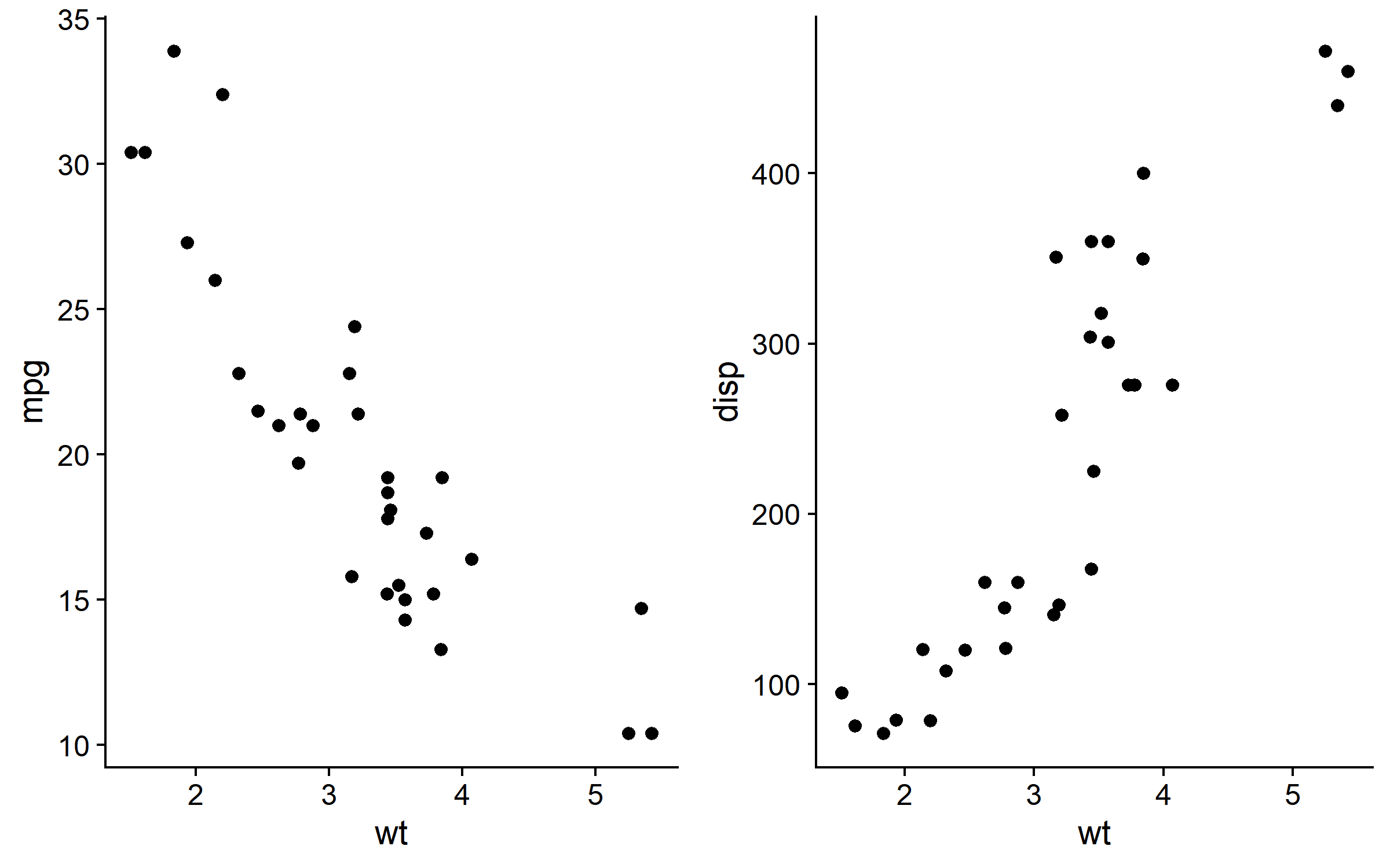
对齐坐标轴
# 不同 y 轴范围的图
pa <- ggplot(mtcars, aes(wt, mpg)) + geom_point() + theme_cowplot()
pb <- ggplot(mtcars, aes(wt, disp)) + geom_point() + theme_cowplot()

# align 参数对齐坐标轴
plot_grid(
  pa, pb,
  ncol = 2,
  align = "h",   # 水平对齐 (h/v/hv/none)
  axis = "bt"    # 对齐哪些轴 (t/b/l/r/tb/lr/tblr)
)
嵌套组合
# 复杂布局:左边一个大图,右边两个小图
right_col <- plot_grid(p2, p3, ncol = 1, labels = c("B", "C"))
plot_grid(p1, right_col, ncol = 2, labels = c("A", ""), rel_widths = c(1.5, 1))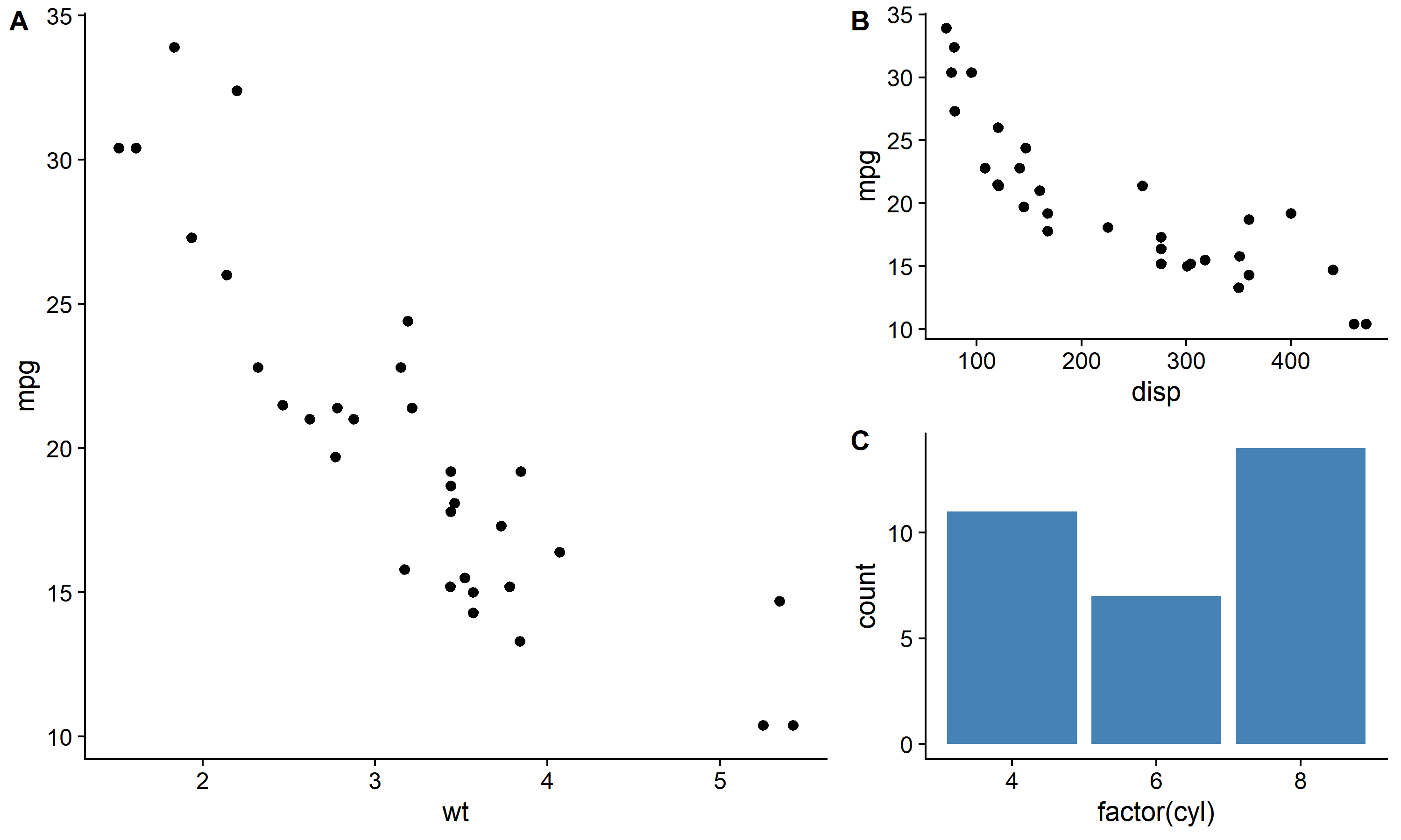
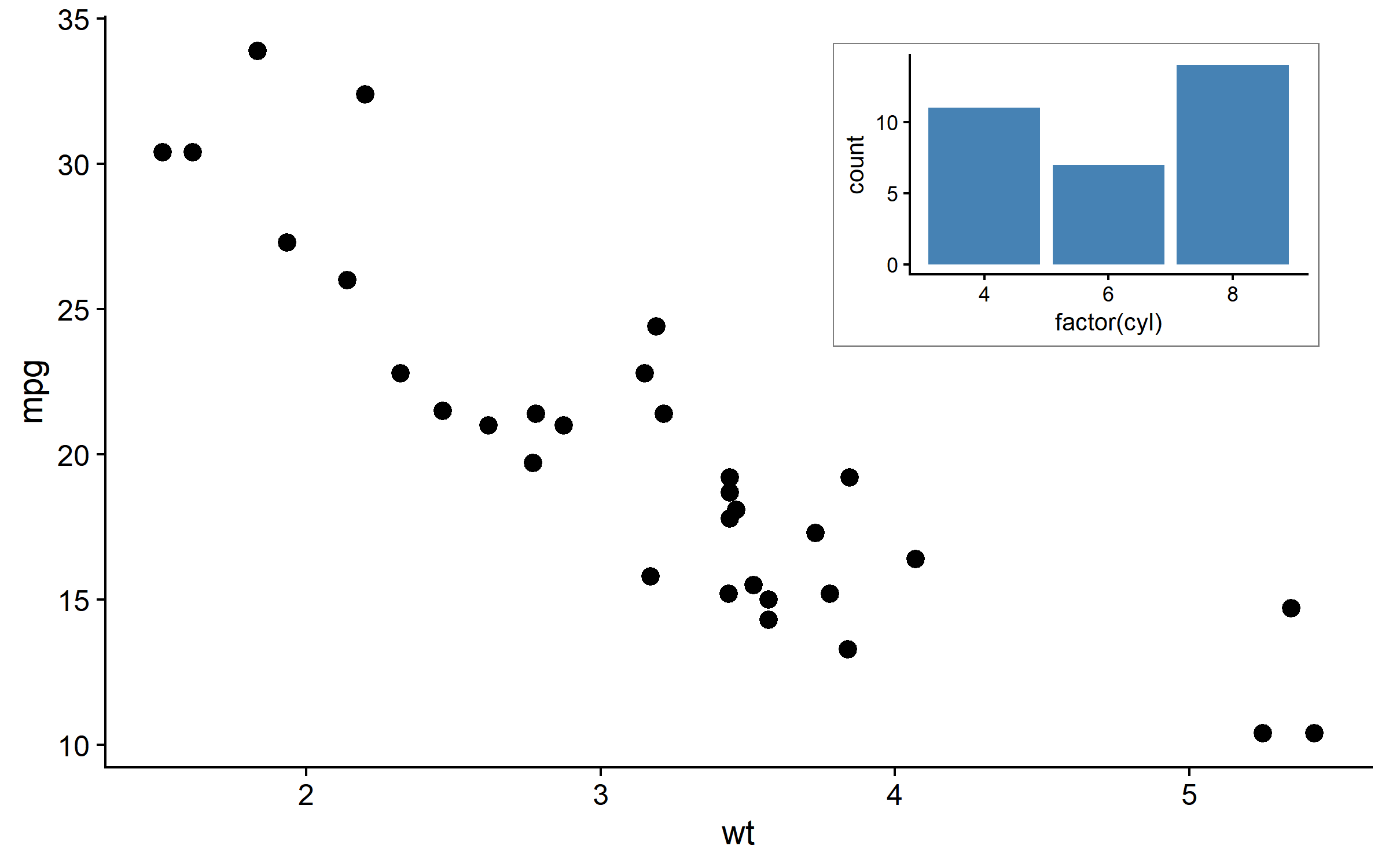
图形嵌入:draw_plot()
在图中嵌入子图
# 主图
main_plot <- ggplot(mtcars, aes(wt, mpg)) +
  geom_point(size = 3) +
  theme_cowplot()

# 子图(缩略图)
inset_plot <- ggplot(mtcars, aes(factor(cyl))) +
  geom_bar(fill = "steelblue") +
  theme_cowplot(font_size = 10) +
  theme(plot.background = element_rect(fill = "white", color = "grey50"))

# 将子图嵌入主图
ggdraw(main_plot) +
  draw_plot(
    inset_plot,
    x = 0.6, y = 0.6,           # 子图左下角位置
    width = 0.35, height = 0.35  # 子图尺寸
  )
多个嵌入图
# 可嵌入多个子图
inset2 <- ggplot(mtcars, aes(hp)) +
  geom_histogram(fill = "coral", bins = 15) +
  theme_cowplot(font_size = 9) +
  labs(title = "HP分布")

ggdraw(main_plot) +
  draw_plot(inset_plot, x = 0.05, y = 0.6, width = 0.3, height = 0.35) +
  draw_plot(inset2, x = 0.65, y = 0.1, width = 0.3, height = 0.3)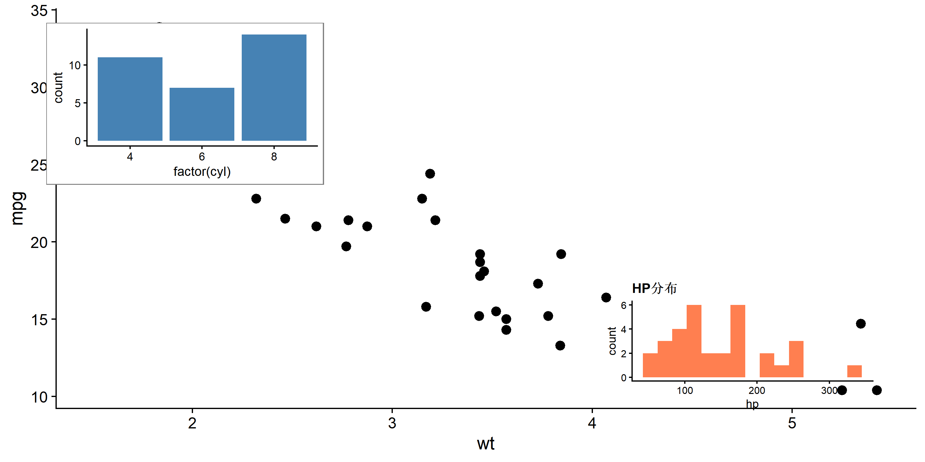
添加注释
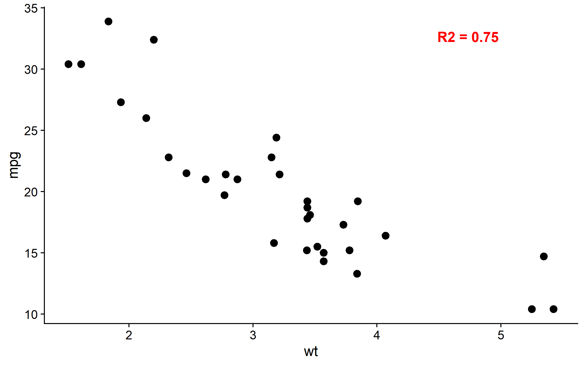
draw_label()
# 添加文字标签
ggdraw(main_plot) +
  draw_label(
    "R2 = 0.75",
    x = 0.8, y = 0.9,
    size = 14,
    fontface = "bold",
    color = "red"
  )
draw_image() - 嵌入图片
# 嵌入外部图片(如 logo)
ggdraw() +
  draw_image("path/to/logo.png", x = 0.4, y = 0.4, width = 0.2) +
  draw_plot(p1)
draw_line() - 添加线条
# 添加参考线或箭头
ggdraw(main_plot) +
  draw_line(x = c(0.2, 0.5), y = c(0.2, 0.8), color = "red", size = 1)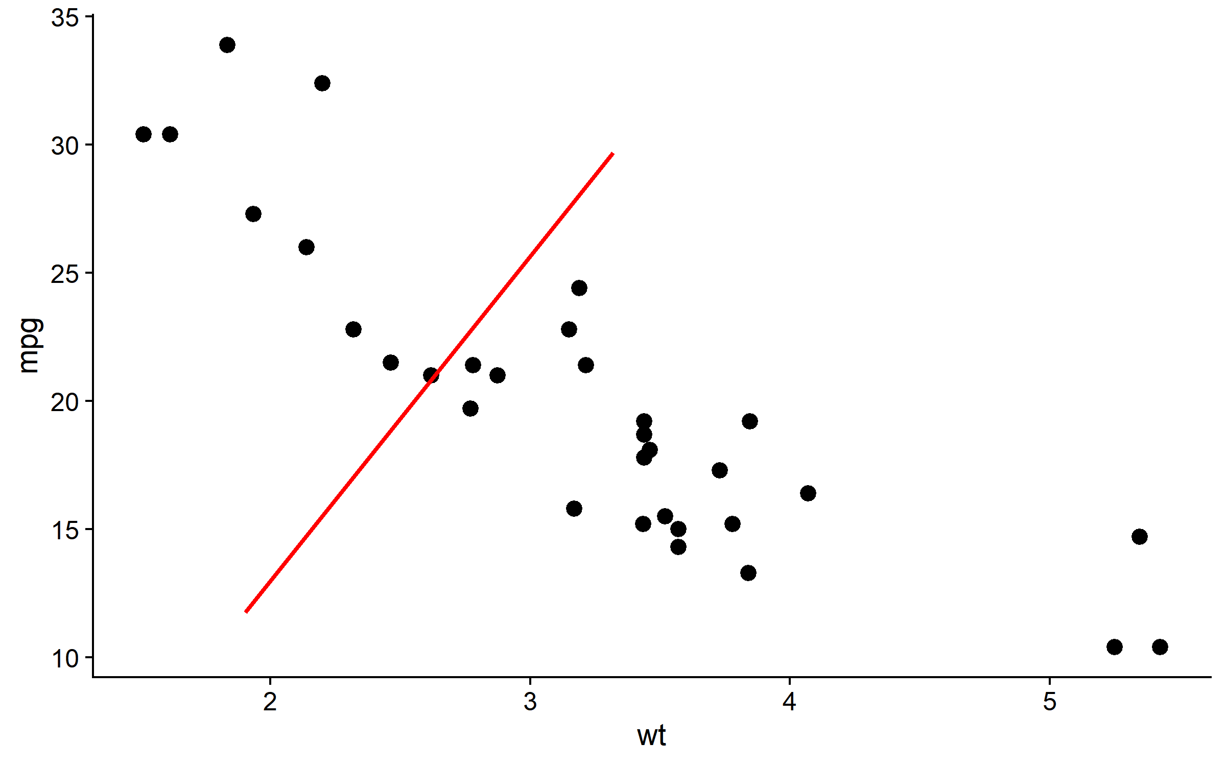
坐标轴对齐:align_plots()
当图形有不同的坐标轴范围时,plot_grid() 的 align 参数可能不够用,此时使用 align_plots() 更精确。
# 两个 y 轴范围差异大的图
plot_a <- ggplot(mtcars, aes(wt, mpg)) + geom_point() + theme_cowplot()
plot_b <- ggplot(mtcars, aes(wt, hp)) + geom_point() + theme_cowplot()

# 精确对齐
aligned <- align_plots(plot_a, plot_b, align = "hv", axis = "tblr")
plot_grid(aligned[[1]], aligned[[2]], ncol = 2)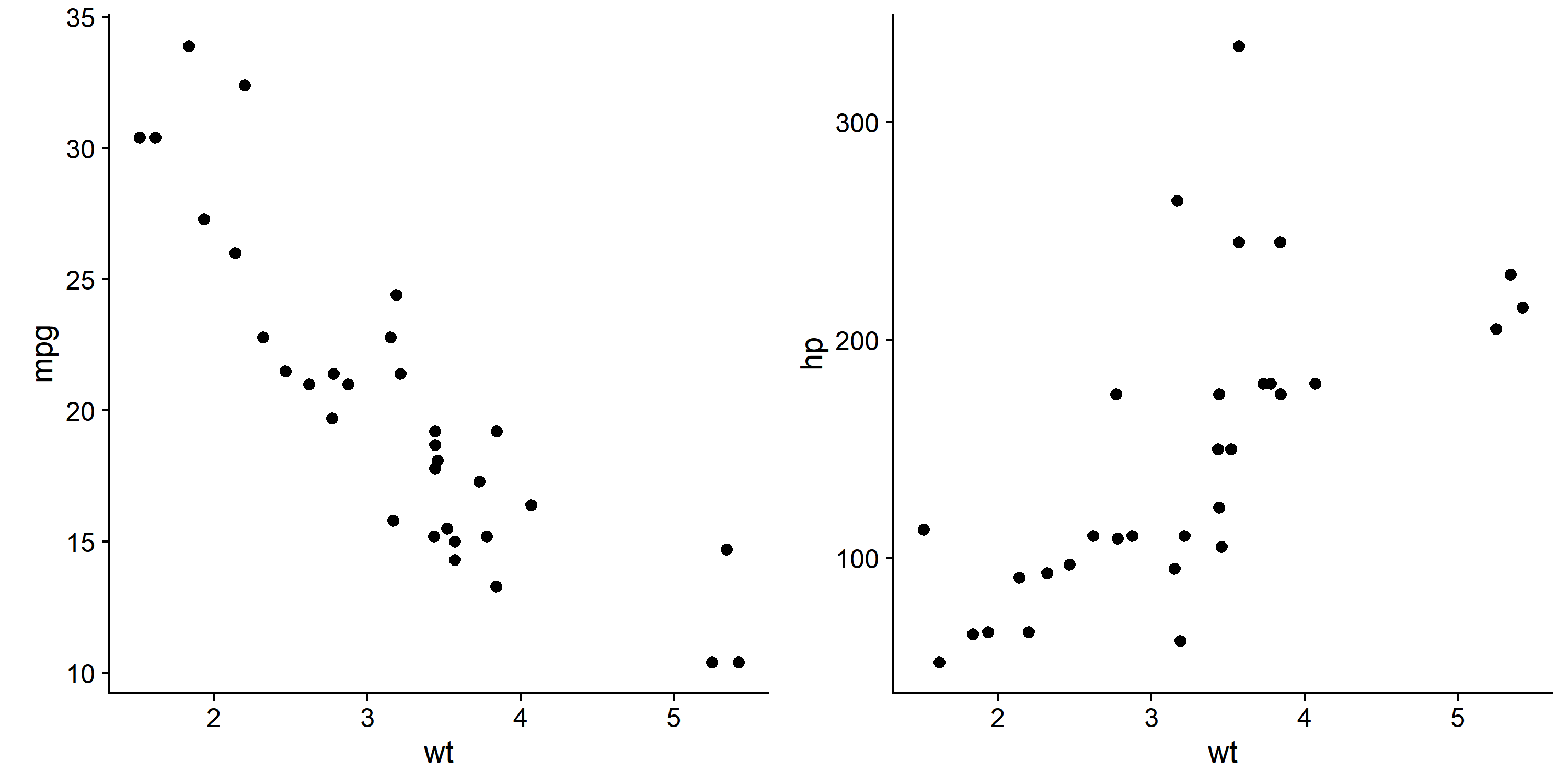
保存组合图
save_plot()
# cowplot 提供的保存函数
combined <- plot_grid(p1, p2, p3, p4, ncol = 2, labels = "AUTO")

# 保存为 PNG
save_plot(
  "combined_plot.png",
  combined,
  ncol = 2,          # 列数(用于计算尺寸)
  nrow = 2,          # 行数
  base_width = 4,    # 每个子图宽度(英寸)
  base_height = 3    # 每个子图高度
)

# 保存为 PDF(矢量图)
save_plot("combined_plot.pdf", combined, ncol = 2, nrow = 2)
ggsave2() - 增强版 ggsave
# ggsave2 自动处理组合图尺寸
ggsave2("output.png", combined, width = 10, height = 8, dpi = 300)
与 ggplot2 facet 对比
| 场景 | 推荐方法 |
|---|---|
| 同一数据的分面 | ggplot + facet_wrap() |
| 不同数据/不同图 | cowplot::plot_grid() |
| 需要不同坐标轴 | cowplot::plot_grid(align = “h”) |
| 需要嵌入子图 | ggdraw() + draw_plot() |
| 复杂嵌套布局 | cowplot 嵌套 plot_grid() |
实战:完整科研图
set.seed(42)
df <- mtcars |> mutate(group = ifelse(mpg > 20, "High", "Low"))

# 图 A: 散点图 + 回归
fig_a <- ggplot(df, aes(wt, mpg)) +
  geom_point(aes(color = group), size = 3) +
  geom_smooth(method = "lm", se = TRUE, color = "grey40") +
  scale_color_manual(values = c("High" = "#E64B35", "Low" = "#4DAF4A")) +
  labs(x = "Weight (1000 lbs)", y = "Miles per Gallon", color = "MPG Group") +
  theme_half_open() +
  theme(legend.position = c(0.8, 0.8))

# 图 B: 箱线图
fig_b <- ggplot(df, aes(factor(cyl), mpg, fill = group)) +
  geom_boxplot() +
  scale_fill_manual(values = c("High" = "#E64B35", "Low" = "#4DAF4A")) +
  labs(x = "Cylinders", y = "MPG", fill = "Group") +
  theme_half_open() +
  theme(legend.position = "none")

# 图 C: 密度图
fig_c <- ggplot(df, aes(mpg, fill = group)) +
  geom_density(alpha = 0.6) +
  scale_fill_manual(values = c("High" = "#E64B35", "Low" = "#4DAF4A")) +
  labs(x = "MPG", y = "Density") +
  theme_minimal_hgrid() +
  theme(legend.position = "none")

# 图 D: 柱状图
fig_d <- df |>
  count(cyl, group) |>
  ggplot(aes(factor(cyl), n, fill = group)) +
  geom_col(position = "dodge") +
  scale_fill_manual(values = c("High" = "#E64B35", "Low" = "#4DAF4A")) +
  labs(x = "Cylinders", y = "Count") +
  theme_half_open() +
  theme(legend.position = "none")

# 组合:上方大图,下方三个小图
top_row <- fig_a
bottom_row <- plot_grid(fig_b, fig_c, fig_d, ncol = 3, labels = c("B", "C", "D"), label_size = 14)

# 最终组合
final_plot <- plot_grid(
  top_row, bottom_row,
  nrow = 2,
  labels = c("A", ""),
  label_size = 14,
  rel_heights = c(1.2, 1)
)

final_plot
与 patchwork 对比
| 特性 | cowplot | patchwork |
|---|---|---|
| 语法 | plot_grid(p1, p2) | p1 + p2 / p1 | p2 |
| 图形嵌入 | draw_plot() | inset_element() |
| 坐标轴对齐 | 需手动 align | 自动对齐 |
| 标签添加 | labels = “AUTO” | plot_annotation(tag_levels) |
| 主题系统 | 丰富的专业主题 | 无 |
| 学习曲线 | 中等 | 简单 |
选择建议:
- 需要专业主题 → cowplot
- 快速组合 → patchwork
- 图形嵌入 → 两者均可
- 复杂布局控制 → cowplot
提取与共享图例
# 创建带图例的图
p_legend <- ggplot(mtcars, aes(wt, mpg, color = factor(cyl))) +
geom_point(size = 3) +
scale_color_brewer(palette = "Set1", name = "Cylinders") +
theme_cowplot()
# 提取图例
legend <- get_legend(p_legend)
# 创建无图例的图
p_no_leg1 <- p_legend + theme(legend.position = "none")
p_no_leg2 <- ggplot(mtcars, aes(disp, mpg, color = factor(cyl))) +
geom_point(size = 3) +
scale_color_brewer(palette = "Set1") +
theme_cowplot() +
theme(legend.position = "none")
# 组合:两图共享一个图例
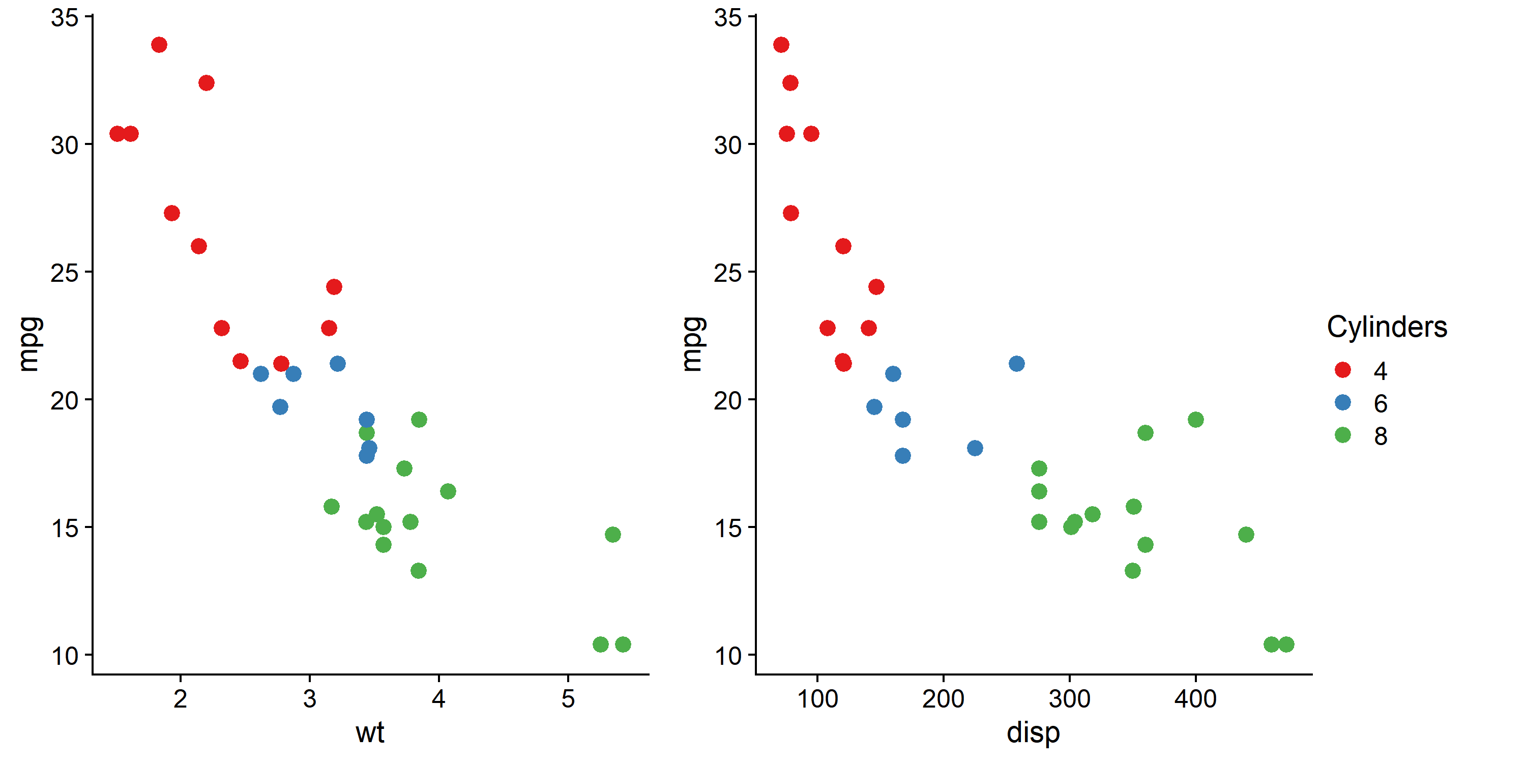
plot_grid(
plot_grid(p_no_leg1, p_no_leg2, ncol = 2),
legend,
ncol = 2,
rel_widths = c(1, 0.15)
)
常用函数速查
| 函数 | 用途 |
|---|---|
| theme_cowplot() | 经典无网格主题 |
| theme_half_open() | 半开放坐标轴 |
| theme_minimal_grid() | 极简网格 |
| plot_grid() | 组合多图 |
| align_plots() | 精确对齐坐标轴 |
| ggdraw() | 创建绑图画布 |
| draw_plot() | 嵌入子图 |
| draw_label() | 添加文字 |
| draw_image() | 嵌入图片 |
| save_plot() | 保存组合图 |
| get_legend() | 提取图例 |
| get_title() | 提取标题 |
总结
cowplot 核心优势:
- 专业主题 - theme_cowplot(), theme_half_open() 直接用于科研图
- 灵活组合 - plot_grid() 支持复杂嵌套布局
- 精确控制 - rel_widths, rel_heights, align 参数
- 图形嵌入 - draw_plot() 轻松添加子图
- 自动标签 - labels = “AUTO” 一键添加面板标签
推荐工作流:
# 1. 创建单图,应用 cowplot 主题
p1 <- ggplot(...) + theme_half_open()
p2 <- ggplot(...) + theme_half_open()

# 2. 组合并添加标签
combined <- plot_grid(p1, p2, labels = "AUTO", align = "hv")

# 3. 保存
save_plot("output.pdf", combined, ncol = 2)