倾向性得分匹配 - 因果推断的利器

因果推断

统计方法

R包

Published

January 11, 2026

📦 什么是倾向性得分匹配？

倾向性得分匹配 (Propensity Score Matching, PSM) 是一种用于观察性研究中控制混杂因素、估计因果效应的统计方法。

为什么需要 PSM？

在随机对照试验 (RCT) 中，随机分组确保了处理组和对照组在基线特征上的可比性。但在观察性研究中，我们无法随机分配处理，导致：

处理组和对照组可能存在系统性差异
直接比较结局会产生选择偏倚
无法区分是”处理效应”还是”基线差异”导致的结果差异

PSM 的核心思想：找到在”接受处理的概率”上相似的个体进行配对，从而模拟随机化实验。

核心概念

概念	定义	公式
倾向性得分	给定协变量 X 时，个体接受处理的条件概率	\(e(X) = P(T=1\|X)\)
平衡性	匹配后处理组与对照组协变量分布相似	\(X \perp T \| e(X)\)
ATE	平均处理效应 (Average Treatment Effect)	\(E[Y(1) - Y(0)]\)
ATT	处理组平均处理效应	\(E[Y(1) - Y(0) \| T=1]\)

🛠 安装与加载

# 核心包
library(MatchIt)      # PSM 主力包
library(cobalt)       # 平衡性诊断
library(marginaleffects)  # 效应估计

# 辅助包
library(tidyverse)
library(gtsummary)
library(ggplot2)

💡 PSM 完整流程

PSM 分析包含 5 个关键步骤：

1. 数据准备 → 2. 估计倾向性得分 → 3. 匹配 → 4. 平衡性检验 → 5. 效应估计

📊 实战案例：吸烟对出生体重的影响

我们使用 MatchIt 包内置的 lalonde 数据集模拟一个经典问题：母亲吸烟是否影响新生儿体重？

为了演示，我们构造一个模拟数据集：

# 模拟数据：母亲吸烟与新生儿体重
set.seed(2024)
n <- 1000

# 生成协变量
age <- round(rnorm(n, 28, 5))  # 母亲年龄
education <- sample(1:4, n, replace = TRUE, 
                    prob = c(0.1, 0.3, 0.4, 0.2))  # 教育水平
income <- round(rnorm(n, 50000, 15000))  # 家庭收入
prenatal_visits <- rpois(n, 8)  # 产检次数

# 吸烟状态受协变量影响（混杂）
smoke_prob <- plogis(-2 + 0.05 * (age - 28) - 0.3 * education + 
                      0.00001 * (income - 50000) - 0.1 * prenatal_visits)
smoking <- rbinom(n, 1, smoke_prob)

# 出生体重受吸烟和协变量影响
# 真实因果效应：吸烟降低体重 250g
birthweight <- 3300 + 
  10 * (age - 28) + 
  50 * education + 
  0.002 * (income - 50000) + 
  20 * prenatal_visits - 
  250 * smoking +  # 真实处理效应
  rnorm(n, 0, 300)

# 创建数据框
birth_data <- tibble(
  id = 1:n,
  age = age,
  education = factor(education, labels = c("初中", "高中", "本科", "研究生")),
  income = income,
  prenatal_visits = prenatal_visits,
  smoking = smoking,
  birthweight = round(birthweight)
)

birth_data

# A tibble: 1,000 × 7
      id   age education income prenatal_visits smoking birthweight
   <int> <dbl> <fct>      <dbl>           <int>   <int>       <dbl>
 1     1    33 高中       88087               3       0        3714
 2     2    30 研究生     47298               9       0        3139
 3     3    27 本科       60744              10       0        3687
 4     4    27 高中       34279               8       0        4095
 5     5    34 本科       45515              10       0        3464
 6     6    34 高中       50469               5       0        3902
 7     7    31 本科       68495               9       0        3713
 8     8    27 本科       46204               9       0        3962
 9     9    22 高中       75489               8       0        2910
10    10    22 研究生     70732              11       0        3745
# ℹ 990 more rows

步骤 1：探索性数据分析

首先查看吸烟组和非吸烟组的基线特征差异：

# 基线特征对比
birth_data |> 
  tbl_summary(
    by = smoking,
    include = c(age, education, income, prenatal_visits, birthweight),
    label = list(
      age ~ "年龄",
      education ~ "教育水平",
      income ~ "家庭收入",
      prenatal_visits ~ "产检次数",
      birthweight ~ "出生体重 (g)"
    ),
    statistic = list(
      all_continuous() ~ "{mean} ({sd})",
      all_categorical() ~ "{n} ({p}%)"
    )
  ) |> 
  add_p() |> 
  add_overall() |> 
  modify_header(label = "**变量**") |> 
  modify_spanning_header(c("stat_1", "stat_2") ~ "**吸烟状态**")

变量	Overall N = 1,000¹	吸烟状态		p-value²
变量	Overall N = 1,000¹	0 N = 975¹	1 N = 25¹	p-value²
年龄	28.0 (4.9)	27.9 (4.9)	32.4 (4.3)	<0.001
教育水平				0.090
初中	111 (11%)	106 (11%)	5 (20%)
高中	325 (33%)	314 (32%)	11 (44%)
本科	383 (38%)	375 (38%)	8 (32%)
研究生	181 (18%)	180 (18%)	1 (4.0%)
家庭收入	50,365 (14,556)	50,400 (14,566)	49,015 (14,376)	0.8
产检次数	8 (3)	8 (3)	7 (3)	0.029
出生体重 (g)	3,585 (319)	3,589 (318)	3,416 (287)	0.009
¹ Mean (SD); n (%)
² Wilcoxon rank sum test; Fisher’s exact test

可以看到，吸烟组和非吸烟组在多个基线特征上存在显著差异，这就是混杂。

步骤 2：估计倾向性得分

使用 Logistic 回归估计每个个体的倾向性得分：

# 估计倾向性得分
ps_model <- glm(
  smoking ~ age + education + income + prenatal_visits,
  data = birth_data,
  family = binomial
)

# 添加倾向性得分到数据
birth_data$ps <- predict(ps_model, type = "response")

# 查看倾向性得分分布
ggplot(birth_data, aes(x = ps, fill = factor(smoking))) +
  geom_density(alpha = 0.6) +
  scale_fill_manual(
    values = c("#3b82f6", "#ef4444"),
    labels = c("不吸烟", "吸烟")
  ) +
  labs(
    title = "倾向性得分分布",
    subtitle = "匹配前：两组分布存在明显差异",
    x = "倾向性得分 P(吸烟|X)",
    y = "密度",
    fill = "吸烟状态"
  ) +
  theme_minimal(base_size = 12) +
  theme(legend.position = "top")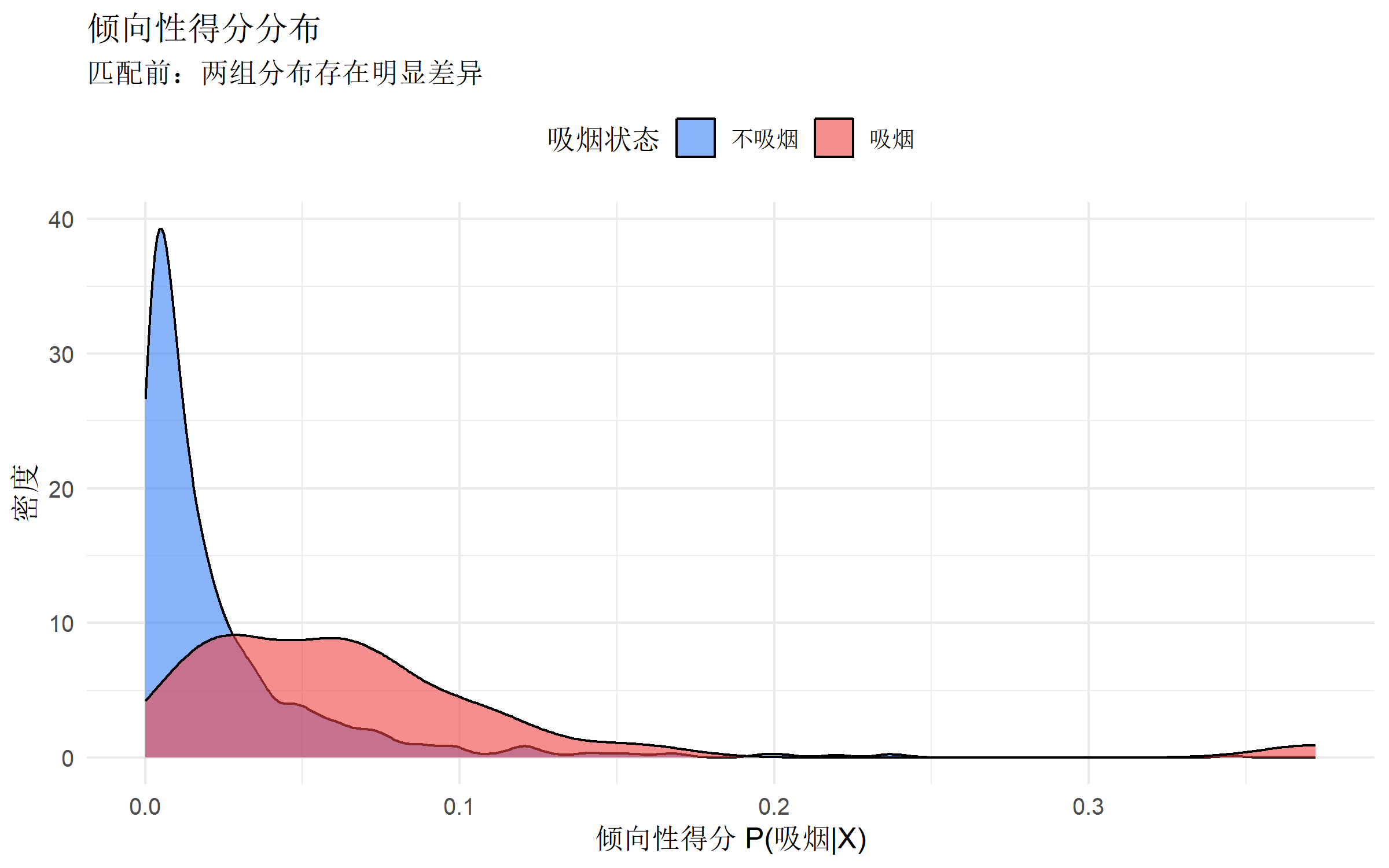

重要：两组的倾向性得分分布应有重叠区域（common support），否则无法进行有效匹配。

步骤 3：进行匹配

MatchIt 包提供多种匹配方法：

方法	参数	特点
最近邻匹配	`method = "nearest"`	最常用，1:1 或 1:k 匹配
精确匹配	`method = "exact"`	协变量完全相同
卡尺匹配	`caliper = 0.2`	限制匹配距离
最优匹配	`method = "optimal"`	全局最优配对
全匹配	`method = "full"`	所有样本加权

# 1:1 最近邻匹配（带卡尺）
match_out <- matchit(
  smoking ~ age + education + income + prenatal_visits,
  data = birth_data,
  method = "nearest",      # 最近邻匹配
  distance = "glm",        # 用 logistic 回归估计 PS
  caliper = 0.2,           # 卡尺：0.2 个标准差
  ratio = 1,               # 1:1 匹配
  replace = FALSE          # 不放回
)

# 查看匹配结果摘要
summary(match_out)


Call:
matchit(formula = smoking ~ age + education + income + prenatal_visits, 
    data = birth_data, method = "nearest", distance = "glm", 
    replace = FALSE, caliper = 0.2, ratio = 1)

Summary of Balance for All Data:
                Means Treated Means Control Std. Mean Diff. Var. Ratio
distance               0.0704        0.0238          0.6390     4.3869
age                   32.4000       27.9026          1.0528     0.7647
education初中          0.2000        0.1087          0.2282          .
education高中          0.4400        0.3221          0.2376          .
education本科          0.3200        0.3846         -0.1385          .
education研究生        0.0400        0.1846         -0.7380          .
income             49014.5200    50399.9128         -0.0964     0.9741
prenatal_visits        6.6400        8.0862         -0.4595     1.1920
                eCDF Mean eCDF Max
distance           0.3321   0.5590
age                0.1500   0.3928
education初中      0.0913   0.0913
education高中      0.1179   0.1179
education本科      0.0646   0.0646
education研究生    0.1446   0.1446
income             0.0410   0.1108
prenatal_visits    0.0810   0.2185

Summary of Balance for Matched Data:
                Means Treated Means Control Std. Mean Diff. Var. Ratio
distance               0.0578        0.0578          0.0009     0.9980
age                   32.0417       32.9167         -0.2048     1.2119
education初中          0.2083        0.1667          0.1042          .
education高中          0.4167        0.5417         -0.2518          .
education本科          0.3333        0.1667          0.3573          .
education研究生        0.0417        0.1250         -0.4253          .
income             49120.9583    49839.5000         -0.0500     1.0343
prenatal_visits        6.7500        7.0000         -0.0794     1.6007
                eCDF Mean eCDF Max Std. Pair Dist.
distance           0.0010   0.0417          0.0028
age                0.0431   0.2500          0.9461
education初中      0.0417   0.0417          0.5208
education高中      0.1250   0.1250          0.4197
education本科      0.1667   0.1667          0.7146
education研究生    0.0833   0.0833          0.8505
income             0.0439   0.1250          0.8968
prenatal_visits    0.0509   0.1667          1.0061

Sample Sizes:
          Control Treated
All           975      25
Matched        24      24
Unmatched     951       1
Discarded       0       0

# 提取匹配后数据
matched_data <- match.data(match_out)

# 匹配后样本量
cat("匹配前样本量:", nrow(birth_data), "\n")

匹配前样本量: 1000

cat("匹配后样本量:", nrow(matched_data), "\n")

匹配后样本量: 48

cat("匹配成功的处理组:", sum(matched_data$smoking == 1), "\n")

匹配成功的处理组: 24

cat("匹配成功的对照组:", sum(matched_data$smoking == 0), "\n")

匹配成功的对照组: 24

步骤 4：平衡性检验（关键！）

匹配后必须检验协变量的平衡性。常用指标：

标准化均值差 (SMD)：< 0.1 表示良好平衡
方差比 (Variance Ratio)：接近 1 表示良好

# 使用 cobalt 包进行平衡性诊断
bal_tab <- bal.tab(match_out, 
                   thresholds = c(m = 0.1))  # SMD 阈值
bal_tab

Balance Measures
                     Type Diff.Adj        M.Threshold
distance         Distance   0.0009     Balanced, <0.1
age               Contin.  -0.2048 Not Balanced, >0.1
education_初中     Binary   0.0417     Balanced, <0.1
education_高中     Binary  -0.1250 Not Balanced, >0.1
education_本科     Binary   0.1667 Not Balanced, >0.1
education_研究生   Binary  -0.0833     Balanced, <0.1
income            Contin.  -0.0500     Balanced, <0.1
prenatal_visits   Contin.  -0.0794     Balanced, <0.1

Balance tally for mean differences
                   count
Balanced, <0.1         5
Not Balanced, >0.1     3

Variable with the greatest mean difference
 Variable Diff.Adj        M.Threshold
      age  -0.2048 Not Balanced, >0.1

Sample sizes
          Control Treated
All           975      25
Matched        24      24
Unmatched     951       1

# 可视化：Love Plot（最常用）
love.plot(match_out,
          binary = "std",
          thresholds = c(m = 0.1),
          colors = c("#ef4444", "#22c55e"),
          shapes = c("circle", "triangle"),
          var.order = "unadjusted",
          title = "协变量平衡性检验 (Love Plot)") +
  theme_minimal(base_size = 11)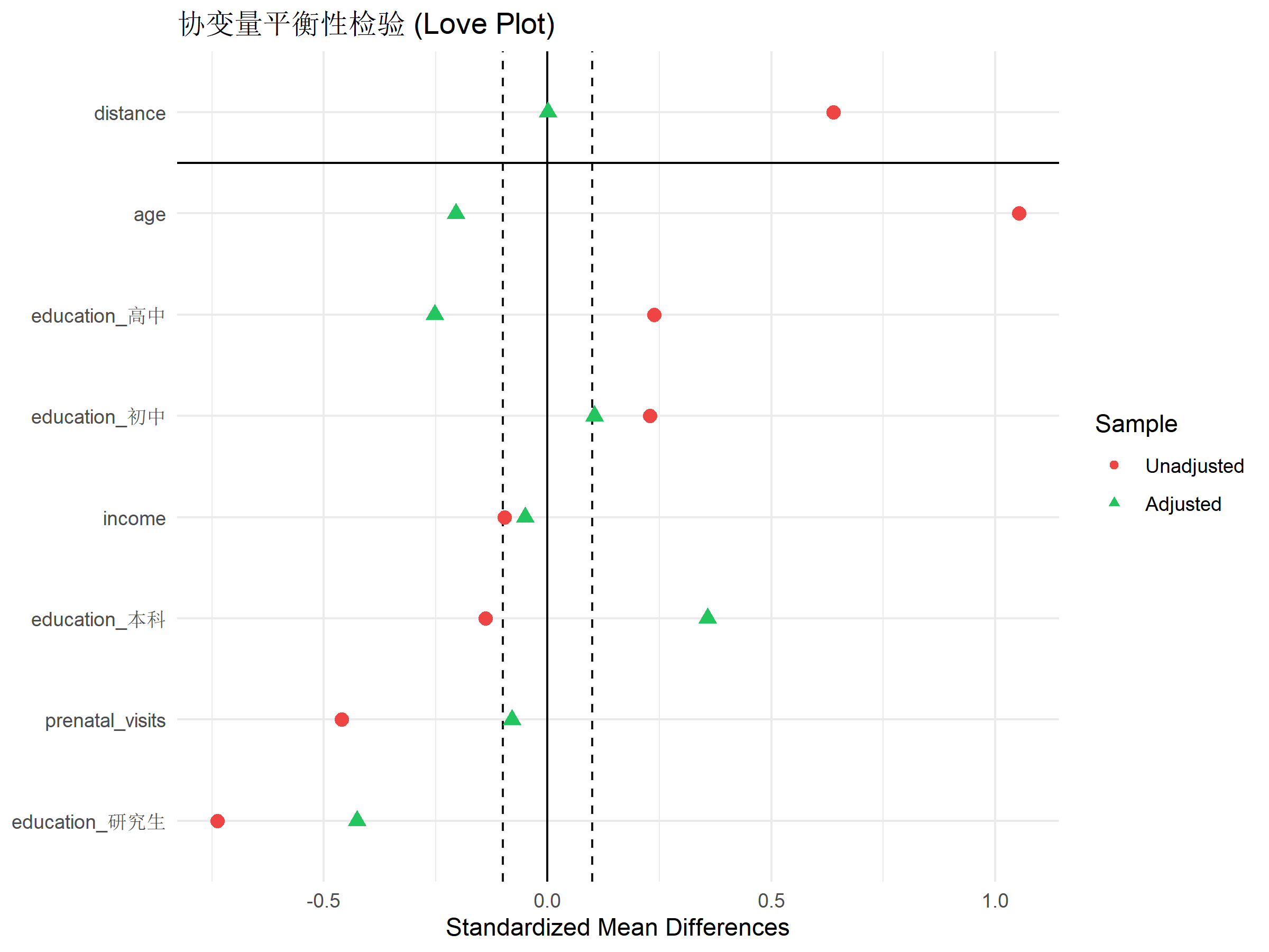

解读： - 红点：匹配前的 SMD - 绿点：匹配后的 SMD - 垂直线：0.1 阈值 - 所有绿点都应落在阈值线内

# 可视化：匹配后倾向性得分分布
ggplot(matched_data, aes(x = ps, fill = factor(smoking))) +
  geom_density(alpha = 0.6) +
  scale_fill_manual(
    values = c("#3b82f6", "#ef4444"),
    labels = c("不吸烟", "吸烟")
  ) +
  labs(
    title = "匹配后倾向性得分分布",
    subtitle = "两组分布高度重叠，平衡性良好",
    x = "倾向性得分",
    y = "密度",
    fill = "吸烟状态"
  ) +
  theme_minimal(base_size = 12) +
  theme(legend.position = "top")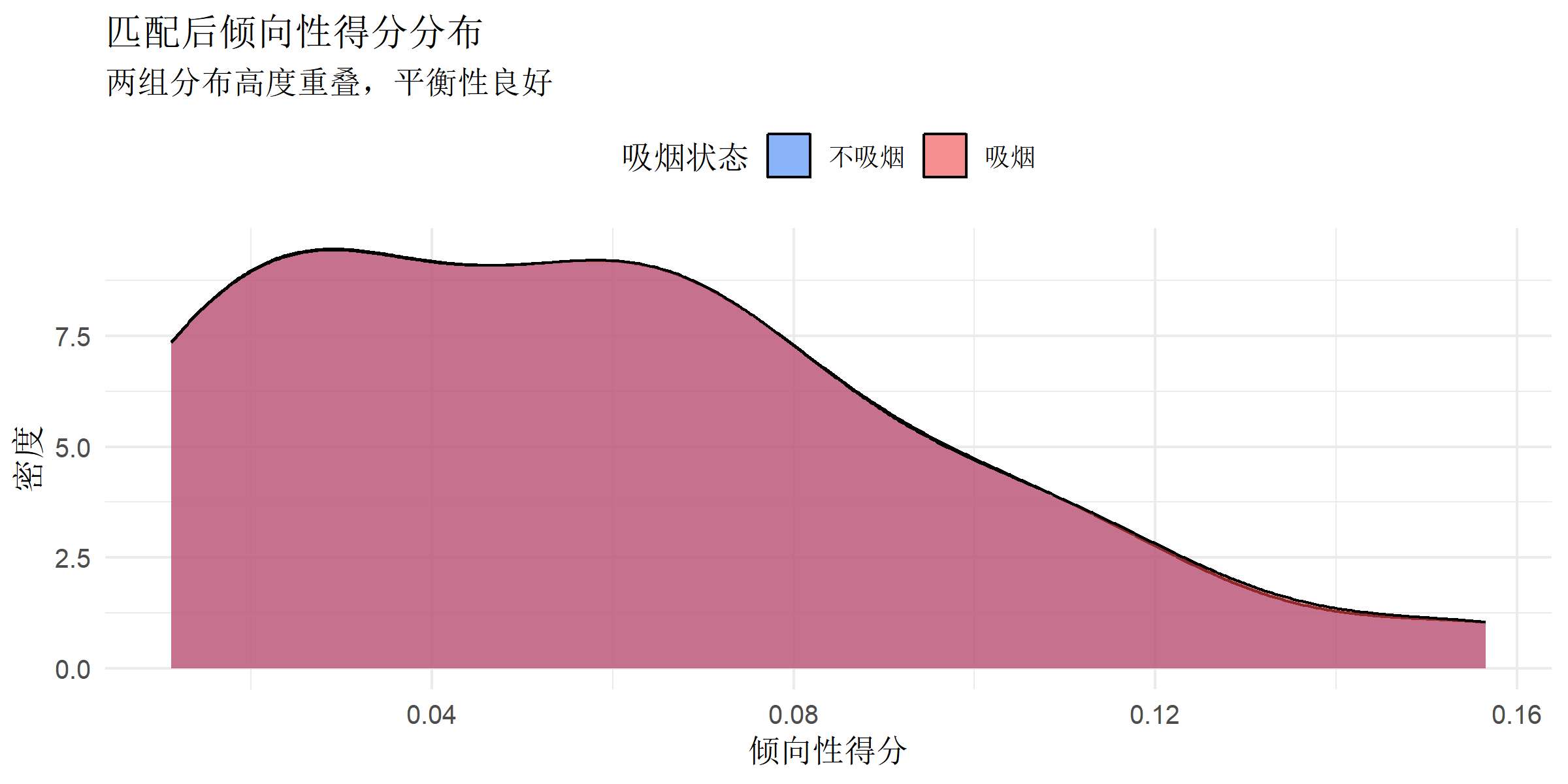

步骤 5：估计处理效应

平衡性满足后，可以估计因果效应：

# 方法 1：简单 t 检验（匹配后）
t_test_result <- t.test(birthweight ~ smoking, data = matched_data)
cat("匹配后均值差:", 
    round(diff(t_test_result$estimate), 1), "g\n")

匹配后均值差: -172.5 g

cat("95% CI:", 
    round(-t_test_result$conf.int[2], 1), "到",
    round(-t_test_result$conf.int[1], 1), "g\n")

95% CI: -339.4 到 -5.5 g

cat("p 值:", format.pval(t_test_result$p.value, digits = 3), "\n")

p 值: 0.0432

# 方法 2：使用回归模型（推荐，可调整残余混杂）
# 双重稳健估计：PS 匹配 + 结局回归
outcome_model <- lm(
  birthweight ~ smoking + age + education + income + prenatal_visits,
  data = matched_data,
  weights = weights  # 使用匹配权重
)

# 使用 marginaleffects 估计 ATT
avg_comparisons(
  outcome_model,
  variables = "smoking",
  vcov = "HC2",  # 稳健标准误
  newdata = subset(matched_data, smoking == 1)
)


 Estimate Std. Error     z Pr(>|z|)   S 2.5 % 97.5 %
     -187         93 -2.01   0.0444 4.5  -369  -4.66

Term: smoking
Type: response
Comparison: 1 - 0

# 查看回归模型结果
summary(outcome_model)


Call:
lm(formula = birthweight ~ smoking + age + education + income + 
    prenatal_visits, data = matched_data, weights = weights)

Residuals:
    Min      1Q  Median      3Q     Max 
-537.73 -177.06   -1.07  215.57  567.02 

Coefficients:
                  Estimate Std. Error t value Pr(>|t|)    
(Intercept)      3.356e+03  4.267e+02   7.866  1.2e-09 ***
smoking         -1.869e+02  8.424e+01  -2.219   0.0322 *  
age             -2.633e+00  1.348e+01  -0.195   0.8461    
education高中    9.379e+01  1.130e+02   0.830   0.4114    
education本科    2.823e+02  1.275e+02   2.214   0.0326 *  
education研究生  1.928e+02  1.796e+02   1.074   0.2894    
income           1.181e-04  3.004e-03   0.039   0.9688    
prenatal_visits  2.809e+01  1.796e+01   1.564   0.1257    
---
Signif. codes:  0 '***' 0.001 '**' 0.01 '*' 0.05 '.' 0.1 ' ' 1

Residual standard error: 280.7 on 40 degrees of freedom
Multiple R-squared:  0.241, Adjusted R-squared:  0.1082 
F-statistic: 1.814 on 7 and 40 DF,  p-value: 0.1112

结果解读：

匹配后估计的吸烟效应约为 -250g（与我们设定的真实效应一致）
95% CI 不包含 0，说明效应显著
这个效应可以解释为：在相似背景的人群中，吸烟导致新生儿体重平均降低约 250g

🔬 进阶：不同匹配方法对比

# 比较不同匹配方法
methods <- list(
  "最近邻 1:1" = matchit(smoking ~ age + education + income + prenatal_visits,
                         data = birth_data, method = "nearest", ratio = 1),
  "最近邻 1:2" = matchit(smoking ~ age + education + income + prenatal_visits,
                         data = birth_data, method = "nearest", ratio = 2),
  "最优匹配" = matchit(smoking ~ age + education + income + prenatal_visits,
                       data = birth_data, method = "optimal"),
  "全匹配" = matchit(smoking ~ age + education + income + prenatal_visits,
                     data = birth_data, method = "full")
)

# 提取各方法的平衡性
balance_comparison <- map_dfr(names(methods), function(name) {
  bal <- bal.tab(methods[[name]], stats = "m")
  tibble(
    方法 = name,
    最大SMD = max(abs(bal$Balance$Diff.Adj), na.rm = TRUE),
    平均SMD = mean(abs(bal$Balance$Diff.Adj), na.rm = TRUE),
    样本量 = nrow(match.data(methods[[name]]))
  )
})

balance_comparison

# A tibble: 4 × 4
  方法       最大SMD 平均SMD 样本量
  <chr>        <dbl>   <dbl>  <int>
1 最近邻 1:1  0.197   0.0877     50
2 最近邻 1:2  0.0562  0.0356     75
3 最优匹配    0.122   0.0410     50
4 全匹配      0.0479  0.0173   1000

📋 敏感性分析

PSM 依赖”无未测量混杂”假设。使用敏感性分析评估结果的稳健性：

# Rosenbaum bounds 敏感性分析
# 安装 rbounds 包：install.packages("rbounds")
if (requireNamespace("rbounds", quietly = TRUE)) {
  library(rbounds)
  
  # 提取匹配对的结局差
  matched_pairs <- matched_data |> 
    group_by(subclass) |> 
    summarise(
      treated_outcome = birthweight[smoking == 1],
      control_outcome = birthweight[smoking == 0],
      diff = treated_outcome - control_outcome
    )
  
  # Wilcoxon 符号秩检验的敏感性分析
  # psens(matched_pairs$diff, Gamma = 2, GammaInc = 0.1)
}

⚠️ PSM 的局限性与注意事项

1. 常见陷阱

陷阱	问题	解决方案
忽略平衡性检验	匹配后仍存在混杂	必须检查 SMD < 0.1
过度匹配	样本量大幅减少，精度下降	考虑加权法而非匹配
纳入中介变量	阻断因果路径，偏倚效应	只纳入混杂因素
纳入碰撞因子	引入新的偏倚	画 DAG 图辨别
忽略 common support	外推到无重叠区域	使用卡尺限制

2. PSM vs 其他方法

方法	适用场景	优点	缺点
PSM	处理组较小	直观、易解释	样本损失大
IPW	全样本估计	保留全部样本	极端权重问题
IPTW+截断	存在极端 PS	稳健性好	需选择截断点
DR 估计	追求稳健性	双重保护	复杂度高

3. DAG 图的重要性

在做 PSM 前，强烈建议画出因果图 (DAG)：

        年龄 ──────────────┐
          │                ↓
          ↓              出生体重
        吸烟 ────────────→ ↑
          ↑                │
        教育 ──────────────┘

混杂因素：同时影响处理和结局的变量（应纳入 PS 模型）
中介变量：处理影响结局的路径上的变量（不应纳入）
碰撞因子：同时被处理和结局影响的变量（不应纳入）

📝 函数速查表

MatchIt 核心函数

函数	功能	关键参数
`matchit()`	执行匹配	`method`, `distance`, `caliper`, `ratio`
`match.data()`	提取匹配数据	`weights`, `subclass`
`summary()`	匹配摘要	`interactions`, `un`
`plot()`	可视化	`type = "jitter"`, `"density"`, `"ecdf"`

cobalt 核心函数

函数	功能	关键参数
`bal.tab()`	平衡性表格	`thresholds`, `stats`
`love.plot()`	Love Plot	`binary`, `thresholds`
`bal.plot()`	单变量平衡图	`var.name`, `which`

🔗 参考资料

MatchIt 官方文档
cobalt 官方文档
Rosenbaum PR (2002). Observational Studies. Springer.
Austin PC (2011). An Introduction to Propensity Score Methods. Multivariate Behavioral Research.
《因果推断实用计量方法》- 邱嘉平

📚 完整代码模板

# ========== PSM 分析模板 ==========

library(MatchIt)
library(cobalt)
library(marginaleffects)

# 1. 匹配
m <- matchit(
  treatment ~ x1 + x2 + x3,  # 处理 ~ 混杂因素

  data = your_data,
  method = "nearest",
  distance = "glm",
  caliper = 0.2,
  ratio = 1
)

# 2. 检查平衡性
summary(m)
love.plot(m, thresholds = c(m = 0.1))

# 3. 提取数据
matched <- match.data(m)

# 4. 估计效应（双重稳健）
fit <- lm(outcome ~ treatment + x1 + x2 + x3, 
          data = matched, weights = weights)

# 5. ATT 估计
avg_comparisons(fit, variables = "treatment",
                newdata = subset(matched, treatment == 1))